EP2630812B1 - Estimation of synthetic audio prototypes - Google Patents
Estimation of synthetic audio prototypes Download PDFInfo
- Publication number
- EP2630812B1 EP2630812B1 EP11776678.2A EP11776678A EP2630812B1 EP 2630812 B1 EP2630812 B1 EP 2630812B1 EP 11776678 A EP11776678 A EP 11776678A EP 2630812 B1 EP2630812 B1 EP 2630812B1
- Authority
- EP
- European Patent Office
- Prior art keywords
- signal
- prototype
- input signals
- audio
- input
- Prior art date
- Legal status (The legal status is an assumption and is not a legal conclusion. Google has not performed a legal analysis and makes no representation as to the accuracy of the status listed.)
- Not-in-force
Links
Images









Classifications
-
- H—ELECTRICITY
- H04—ELECTRIC COMMUNICATION TECHNIQUE
- H04S—STEREOPHONIC SYSTEMS
- H04S3/00—Systems employing more than two channels, e.g. quadraphonic
- H04S3/02—Systems employing more than two channels, e.g. quadraphonic of the matrix type, i.e. in which input signals are combined algebraically, e.g. after having been phase shifted with respect to each other
-
- H—ELECTRICITY
- H04—ELECTRIC COMMUNICATION TECHNIQUE
- H04S—STEREOPHONIC SYSTEMS
- H04S2400/00—Details of stereophonic systems covered by H04S but not provided for in its groups
- H04S2400/05—Generation or adaptation of centre channel in multi-channel audio systems
-
- H—ELECTRICITY
- H04—ELECTRIC COMMUNICATION TECHNIQUE
- H04S—STEREOPHONIC SYSTEMS
- H04S2400/00—Details of stereophonic systems covered by H04S but not provided for in its groups
- H04S2400/15—Aspects of sound capture and related signal processing for recording or reproduction
-
- H—ELECTRICITY
- H04—ELECTRIC COMMUNICATION TECHNIQUE
- H04S—STEREOPHONIC SYSTEMS
- H04S2420/00—Techniques used stereophonic systems covered by H04S but not provided for in its groups
- H04S2420/07—Synergistic effects of band splitting and sub-band processing
Definitions
- This invention relates to estimation of synthetic audio prototypes.
- upmixing generally refers to the process of undoing "downmixing", which is the addition of many source signals into fewer audio channels.
- Downmixing can be a natural acoustic process, or a studio combination.
- upmixing can involve producing a number of spatially separated audio channels from a multichannel source.
- the simplest upmixer takes in a stereo pair of audio signals and generates a single output representing the information common to both channels, which is usually referred to as the center channel.
- a slightly more complex upmixer might generate three channels, representing the center channel and the "not center” components of the left and right inputs. More complex upmixers attempt to separate one or more center channels, two "side-only” channels of panned content, and one or more "surround” channels of uncorrelated or out of phase content.
- One method of upmixing is performed in the time domain by creating weighted (sometimes negative) combinations of stereo input channels. This method can render a single source in a desired location, but it may not allow multiple simultaneous sources to be isolated. For example, a time domain upmixer operating on stereo content that is dominated by common (center) content will mix panned and poorly correlated content into the center output channel even though this weaker content belongs in other channels.
- a number of stereo upmixing algorithms are commercially available, including Dolby Pro Logic II (and variants), Lexicon's Logic 7 and DTS Neo:6, Bose'sVideostage, Audio Stage, Centerpoint, and Centerpoint II.
- the present invention relates to a method for forming one audio output signal from a plurality of audio input signals, as recited in claim 1.
- Advantageous embodiments are set out in dependent claims of the appended set of claims.
- an example of a system that makes use of estimation of synthetic prototypes is an upmixing system 100 that includes an upmix module 104, which accepts input signals 112 s 1 ( t ),..., s N ( t ) and outputs an upmixed signal d ⁇ ( t ) .
- upmix module 104 accepts input signals 112 s 1 ( t ),..., s N ( t ) and outputs an upmixed signal d ⁇ ( t ) .
- input time signals s 1 ( t ) and s 2 ( t ) represent left and right input signals
- d ⁇ (t) represents a derived center channel.
- the upmix module 104 forms the upmixed signal d ⁇ ( t ) as a combination of the input signals s 1 ( t ),..., s N ( t ) 112, for instance as a (time varying) linear combination of the input signals.
- the upmixed signal d ⁇ (t) is formed by an estimator 110 as a linear estimate of the prototype signal d(t) 109, which is formed from the input signals by a prototype generator 108, generally by a non-linear technique.
- the estimate is formed as a linear (e.g., frequency weighted) combination of the input signals that best approximates the prototype signal in a minimum mean-squared error sense.
- This linear estimate d ⁇ (t) is generally based on a generative model 102 for the set of input signals 112 as being formed as a combination of an obscured target signal d ⁇ (t) and noise components 114 each associated with one of the input signal 112.
- a synthetic prototype generation module 108 forms the prototype d ( t ) 109 as nonlinear transformations of the set of input signals 112. It should be recognized that the prototype can also be formed using linear techniques, as an example, with the prototype being formed from a different subset of the input signals than is used to estimate the output signal from the prototype. For certain types of prototype generation, the prototype may include degradation and/or artifacts that would produce low quality audio output if presented directly to a listener without passing through the linear estimator 110. As introduced above, in some examples, the prototype d ( t ) is associated with a desired upmixing of input signals. In other examples, the prototype is formed for other purposes, for example, based on an identification of a desired signal in the presence of interference.
- the process of forming the prototype signal is more localized in time and/or frequency than is the estimation process, which may introduce a degree of smoothness that can compensate for unpleasant characteristics in the prototype signal resulting from the localized processing.
- the local nature of the prototype generation provides a degree of flexibility and control that enables forms of processing (e.g., upmixing) that are otherwise unattainable.
- the upmixing module 104 of the upmixing system 100 illustrated in FIG. 1 is implemented by breaking each input signal 112 into components (e.g., frequency bands) and processing each component individually.
- the linear estimator 110 can be implemented by independently forming an estimate of each orthogonal component, and then synthesizing the output signal from the estimated components. It should be understood that although the description below focuses on components formed as frequency bands of the input signals, other decompositions into orthogonal or substantially independent components may be equivalently used.
- Such alternative decomposition may include Wavelet transform of the input signals, non-uniform (e.g., psychoacoustic critical bands; octaves) filter banks, perceptual component decomposition, quadrature mirror filterbanks, statistical (e.g., principal components) based decompositions, etc.
- non-uniform e.g., psychoacoustic critical bands; octaves
- perceptual component decomposition e.g., quadrature mirror filterbanks
- statistical e.g., principal components
- an upmixing module 104 is configured to process decompositions of the input signals (in this example two input signals) in a manner similar to that described in U.S. Patent 7,630,500 , titled "Spatial Disassembly Process,".
- Each of the input signals 112 is transformed into a multiple component representation with individual components 212.
- the input signal s 1 ( t ) is decomposed into a set of components s 1 i t indexed by i.
- component analyzer 220 is a discrete Fourier transform (DFT) analysis filter bank that transforms the input signals into frequency components.
- the frequency components are outputs of zero-phase filters, each with an equal bandwidth (e.g., 125Hz).
- the output signal d ⁇ (t) is reconstructed from a set of components d ⁇ i ( t ) using a reconstruction module 230.
- the component analyzers 220 and the reconstruction module 230 are such that if the components are passed through without modification, the originally analyzed signal is essentially (i.e., not necessarily perfectly) reproduced at the output of the reconstruction module 230.
- the component analyzer 220 windows the input signals 112 into time blocks of equal size, which may be indexed by n .
- the blocks may overlap (i.e., part of the data of one block may also be contained in another block), such that each window is shifted in time by a "hop size" ⁇ .
- a windowing function e.g., square root Hanning window
- the component analyzer 220 may zero pad each block of the input signals 112 and then decompose each zero padded block into their respective component representations.
- the components 212 form base band signals, each modulated by a center frequency (i.e., by a complex exponential) of the respective center frequencies of the filter bands. Furthermore each component 212 may be downsampled and processed at a lower sampling rate sufficient for the bandwidth of the filter bands. For example, the output of a DFT filter bank band-pass filter with a 125Hz bandwidth may be sampled at 250Hz without violating the Nyquist criterion.
- the windowed frame forms the input to a 1024_point FFT.
- Each frequency component is formed from one output of the FFT. (Other windows may be chosen that are shorter of longer than the input length of the FFT. If the input window is shorter than the FFT, the data can be zero-extended to fit the FFT; if the input window is longer than the FFT, the data can be time-aliased.)
- one approach to synthesis of prototype signals is on a component-by-component basis, and in particular in a component-local basis such that each component for each window period is processed separately to form one or more prototypes for that local component.
- a component upmixer 206 processes a single pair of input components, s 1 i t and s 2 i t to form an output component d ⁇ i (t).
- the component upmixer 206 includes a component-based local prototype generator 208 which determines a prototype signal component d i (t) (typically at the downsampled rate) from the input components s 1 i t and s 2 i t .
- the prototype signal component is a non-linear combination of the input components.
- a component-based linear estimator 210 estimates the output component d ⁇ i ( t ).
- the local prototype generator 208 can make use of synthesis techniques that offer the possibility to perform a wide range of transforms that might not otherwise be possible by using linear processing techniques alone. For example, upmixing, modification of room acoustics, and signal selection (e.g., for telephones and hearing aids) can all be accomplished using this class of synthetic processing techniques.
- the local prototype signal is derived based on knowledge, or an assumption, about the characteristics of the desired signal and undesired signals, as observed in the input signal space. For instance, the local prototype generator selects inputs that display the characteristics of the desired signal and inhibits inputs that do not display the desired characteristics.
- selection means passing with some pre-defined maximum gain, example unity, and in the limit, inhibition means passing with zero gain.
- Preferred selection functions may have a binary characteristic (pass region with unity gain, reject region with zero gain) or a gentle transition between passing signals with desired characteristics and rejecting signals with undesired characteristics.
- the selection function may include a linear combination of linearly modified inputs, one or more nonlinearly gated inputs, multiplicative combinations of inputs (of any order) and other nonlinear functions of the inputs.
- the synthetic prototype generator 208 generates what are effectively instantaneous (i.e., temporally local) "guesses" of signal desired at the output, without necessarily considering whether a sequence of such guesses would directly synthesize an artifact-free signal.
- approaches described in U.S. Patent 7,630,500 that are used to compute components of an output signal are used in the present approaches to compute components of a prototype signal, which are then subject to further processing.
- the present approaches may differ from those described in the referenced patent in characteristics such as the time and/or frequency extent of components. For instance, in the present approach, the window "hop rate" may be higher, resulting a more temporally local synthesis of prototypes, and in some synthesis approaches, such a higher hop rate might result in more artifacts if the approaches described in the referenced patent were used directly.
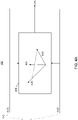
- one exemplary multiple input local prototype d i ( t ) generator 408 (an instance of the non-linear prototype generator 208 shown in FIG. 2 ) for a center channel is illustrated in the complex plane for a single time value.
- the input signals 412, s 1 i t and s 2 i t are complex signals due to their base-band representations.
- the above formula indicates that the center local prototype d i ( t ) is the average of equal-length parts of the two complex input signals 412. In other words, of the two inputs 412, the one with the larger magnitude is scaled by a real coefficient to match the length of the smaller, and then the average of the two is taken.
- This local prototype signal has a selection characteristic such that its output is largest in magnitude when the two inputs 412 are in phase and equal in level, and it decreases as the level and phase differences between the signals increase. It is zero for "hard-panned" and phase-reversed left and right signals. Its phase is the average of the phase of the two input signals.
- the vector gating function can generate a signal that has a different phase than either of the original signals, even though the components of the vector gating factor are real-valued.
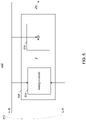
- a prototype generation module 508 (which is another instance of the prototype generator 208 shown in FIG. 2 ) includes a gating function 524 and a scaler 526.
- the gating function 524 module accepts the input signals 512 and uses them to determine a gating factor g i , which is kept constant during the analysis interval corresponding to one windowing of the input signal.
- the gating function module 524 may be switched between 0 and 1 based on the input signals 512.
- the gating function module 524 may implement a smooth slope, where the gating is adjusted between 0 and 1 based on the input signals 512 and/or their history over many analysis windows.
- One of the input signals 512 for instance s 1 i t , and gating factor g are applied to scaler 526 to yield local prototype d(t) .
- This operation dynamically adjusts the amount of input signal 512 that is included in the output of the system. Because g is a function of s 1 , d ( t ) is not a linear function of s 1 , and is thus the local prototype is a non-linear modification of s 1 that has a dependency on s 2 . Because the gating factor is real only, the local prototype, d , has the same phase as s 1 ; only its magnitude is modified. Note that the gating factor is determined on a component-by-component basis, with the gating factor for each band being adjusted from analysis window to analysis window.
- the headset may include two microphones configured to be spaced apart from one another and substantially co-linear with the primary direction of acoustic propagation of the speaker's voice.
- the microphones provide the input signals 512 to the prototype generation module 508.
- the gating function module 524 analyzes the input signals 512 by, for example, observing the phase difference between the two microphones. Based on the observed difference, the gating function 524 generates a gating factor g i for each frequency component i.
- the gating factor g i may be 0 when the phase at both microphones is equal, indicating that the recorded sound is not the speaker's voice and instead an extraneous sound from the environment.
- the gating factor may be 1.
- the gating function is configured for use in a hearing assistance device in a manner similar to that described in U.S. Patent Pub. 2009/0262969 , titled “Hearing Assistance Apparatus", which is incorporated herein by reference.
- the gating function is configured to provide more emphasis to a sound source that a user is facing than a sound source that a user is not facing.
- the gating function is configured for use in a sound discrimination application in which the prototype is determined in a manner similar to the way that output components are determined in U.S. Patent Pub. 2008/0317260 , titled “Sound Discrimination Method and Apparatus," which is incorporated herein by reference.
- the output of the multiplier (42) which is the product of an input and a gain (40) (i.e., gating term) in the referenced publication, is applied as a prototype in the present approaches.
- the estimator 110 is configured to determine the output d ⁇ (t) that best matches a prototype d(t).
- the estimator 110 is a linear estimator that matches d ⁇ ( t ) in a least squares sense. Referring back to FIG. 2 , for at least some forms of estimator 110, this estimate may be performed on a component by component basis because generally, the errors in each component are uncorrelated resulting from the orthogonality of the components, and therefore each component can be estimated separately.
- the weights w i are chosen for each analysis window by a least squares weight estimator 216 to form lowest error estimate based on auto and cross power spectra of the input signals s 1 ( t ) and s 2 (t) .
- the computation implemented in some examples of the estimation module may be understood by considering a desired (complex) signal d ⁇ ( t ) and a (complex) input signal x ( t ) with the goal being to find the real coefficient h such that
- a time averaging or filtering over multiple time windows may be used.
- Other causal or lookahead, finite impulse response or infinite impulse response, stationary or adaptive, filters may be used. Adjustment with the factor ⁇ is then applied after filtering.
- FIG. 6 one embodiment 700 of the least squares weight estimation module 216 is illustrated for the case of estimating a weight h for forming the prototype based on a single component.
- the component of the input is identified as X in the figure (e.g., a component s i ( t ) downsampled to a single sample per window), and the prototype component is identified as D in the figure.
- FIG. 6 represents a discrete time filtering approach that is updated once every window period.
- S DX is calculated along the top path by computing the complex conjugate 750 of X, multiplying 752 the complex conjugate of X by D, and then low-pass filtering 754 that product along the time dimension. The real part of S DX is then extracted.
- S XX is calculated along the bottom path by squaring the magnitude 760 of X and then low-pass filtering 762 the result along the time dimension. A small value ⁇ is then added 764 to S XX to prevent division by zero. Finally, h is calculated by dividing 758 Re ⁇ S DX ⁇ by S XX + ⁇ .
- the computation implemented by the estimation module may be further understood by considering a desired signal d ( t ) formed as combination of two inputs x(t) and y(t) with the goal being to find the real coefficients h and g such that
- the using real coefficients is not necessary, and in alternative embodiments with complex coefficients, the formulas for the coefficient values are different (e.g., for complex coefficients, the Re( ) operation is dropped on all terms).
- each of the auto- and cross-correlation terms are filtered over a range of windows and adjusted prior to computation.
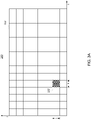
- FIG. 3A is a graphical representation 300 of a time-component representation 322 for all the input channels s k ( t ) and the one or more prototypes d ( t ) .
- Each tile 332 in the representation 300 is associated with one window index n and one component index i .
- FIG. 3B is a detailed view of a single tile 332. In particular FIG. 3B shows that the tile 332 is created by first time windowing 380 each of the input signals 312. The time windowed section of each input signal 312 is then processed by a component decomposition module 220.
- each tile 332 an estimate of the auto 384 and cross 382 correlations of the input channels 312, as well as cross correlations 382 of each of the inputs and each of the outputs is computed, and then filtered 386 over time and adjusted to preserve numerical stability. Then each of the weighting coefficients w k i are computed according a matrix formula of the form shown above.
- the smoothing of the correlation coefficients is performed over time.
- the smoothing is also across components (e.g., frequency bands).
- the characteristics of the smoothing across components may not be equal, for example, with a larger frequency extent at higher frequencies than at lower frequencies.
- the dependence on the time variable t is omitted. Note that for some selections of analysis period ⁇ , only a single value is needed to represent the component, and therefore omitting the dependence on t can be considered as corresponding to a single (complex) value representing the analysis component. Also, in general, the weighting values are generally complex rather than real as is the case in certain examples presented above.
- d is a local time-frequency estimate of a desired signal (i.e., a desired prototype) and the goal is to find the vector w such that the local weighted combination of the inputs (i.e., w T x ) best fits d in a least squared error sense.
- the resulting least squares estimate of d has a smoothing effect on d which can be perceptually pleasing to a listener.
- d ⁇ can better retain the desired behavior of d than a simply smoothed version of d.
- a short-time implementation of the least squares solution is optionally implemented by applying low pass filters (i.e., short time expectation operators and/or cross-frequency smoothing of the statistics) to the cross and auto statistics of the closed-form solution to w.
- low pass filters i.e., short time expectation operators and/or cross-frequency smoothing of the statistics
- the short-time implementation of least squares solution can be extended and applied to a variety of other problems (e.g., dynamic filter coefficients) by adding constraints.
- it can be seen as a short-time implementation of a time-varying closed form least-squares solution. This time-varying closed form least-squares solution can be applied to a variety of other situations.
- the prototype estimate for a frequency component i at a time frame n is assumed to depend on input signals at that same component and frame index, and possibly indirectly on other components and time frames by smoothing of the statistics used in estimation. More generally, a prototype d n at time frame n (or more precisely a prototype d n,i for frequency component i at time frame n ; but the dependence on i is omitted for simplicity of notation) depends on inputs x n , ⁇ , x n-k +1 over a range of k time frames n - k +1, ⁇ , n , and each input x i can be a vector of values that includes other frequency components than that of the prototype being estimated.
- a system 800 receives an input signal x n where n is, for example, the n th frame of the input signal.
- the prototype generator 802 utilizes multiple past inputs of the input component x n or past prototype estimates y n- 1 ⁇ y n-k to determine the prototype signal component d n at time n .
- R z is ( k + / + 1) column vector of input signals
- R z is ( k + / + 1) by (.. k + l +1 ..), so that for many input signals the inversion of R 2 could be expensive.
- the output of the component based linear estimator 804, w is passed to a linear combination module 806 (e.g., an IIR filter) which forms the estimate d ⁇ as a combination of the past input and past output values of x n in the same manner as the prototype generator 802.
- the linear combination module 806 uses the values included in the w vector in place of the b 0 , b 1 , ⁇ , b k and a 1 , a 2 , ⁇ , a l values (i.e., replace b 0 with w b 0 , b 1 with w b 1 , and so on).
- the output of the linear combination module 806, d ⁇ n is the lowest error estimate of d n .
- each prototype is a different time frame (i.e., delay) of a particular signal component, then it may be desirable that the filtering of input components at different lags be time invariant.
- Another example is presented in Section 5.7 below.
- the input signals combined using w may be different for each desired prototype signal in d .
- each input value is effectively deemed to have the same importance in the determination of the prototype estimate by virtue of effectively minimizing the sum of the squares of the e i .
- Including this matrix in the least squares solutions described above causes an error due to a higher weighted input constraint to cost more than an error due to a lower weighted input constraint. This biases the least squares solution toward constraints with greater weights.
- the constraint weights vary with time and/or frequency and can be driven by other information within a system. In other examples, there can be situations within a given frequency band where one constraint should take precedence over another, and vice versa.
- the goal is to find the linear combination of two input channel signals at time index n, x 1, n and x 2, n , that is the best estimate d ⁇ n of the desired signal d n at time n n .
- d d n
- Z x 1 n
- x 2 n x 1 n
- E Z H d E x 1 n x 2 n ⁇ x 1 n x 2 n ⁇ 1 E x 1 n x 2 n ⁇ d n
- This example differs from Example 1 in that instead of using two different channels as input, two different time segments of a single channel are used as input. The goal is find the linear combination of the current (at time n ) and previous (at time n -1) input signals, x n and x n -1 , that is the best estimate d ⁇ n of the desired signal d n at the current time n .
- Examples 1 and 2 illustrate that it is possible to solve for the local desired signal d n by taking inputs across both channels and/or time.
- the dimension P becomes greater than two and inverting a P ⁇ P matrix Z H Z can be expensive.
- additional desired signals (which correspond to additional input constraints, i.e. the dimension N ) can be used without increasing the size of the PxP matrix inversion.
- least squares smoothing is applied to a microphone array.
- the raw signals from the microphones in the array are used to estimate a desired source signal component at specific points in time and frequency.
- the goal is to determine a linear combination of the microphone signals which best approximates an instantaneous desired signal at the specific points in time and frequency.
- the least squares solution may not only provide the desired smoothing behavior to the desired signal, but can also produce coefficients which provide cancellation when the coefficients solved are complex valued.
- a source 1002 at an ideal or known source location produces a source signal (e.g., an audio signal) which propagates through the air to each microphone 1004 of a microphone array 1006 that includes in this example two microphones, M1 and M 2.
- a source signal e.g., an audio signal
- H dp the transfer function of a particular signal component (e.g., frequency band) is referred to as h dp .
- One example of such a situation is in the case of an ear-mounted microphone array in which the location of the mouth is known (at least approximately) relative to the microphones, and therefore the transfer function may be predetermined or estimated during use.
- Another preferable approach is to form the prototype estimates from the separate input signals in such a way that the weighting of the input signals approximately (but not necessarily) matches the known transfer functions from the ideal source location. In this way, a signal arriving from the ideal source location is generally passed without modification.
- d [ d n ,1] T .
- the above solution combines a time invariant constraint with a time-varying solution.
- the additional constraint can be used to help restrain the instantaneous solution for w based on estimating d n alone from substantially harming any source signal that originated from the ideal source location. Note, however, that this is not an absolute constraint as is the case for the MVDR solution (which strictly forbids any distortion in the target source direction).
- the above example can be extended to include an additional constraint such that the instantaneous coefficients w produce a null in a particular direction with respect to the microphone array 1106.
- the direction can be expressed as a transfer function H np (where p is the p th microphone) between a noise (or otherwise not desired) source, N 1108 at an ideal or known noise location and the P microphones 1104 in the microphone array 1106.
- H np the transfer function between a noise (or otherwise not desired) source, N 1108 at an ideal or known noise location
- the transfer function of a signal component e.g., a frequency band
- h np the transfer function of a signal component
- the weighted solution for this example produces a tendency towards a null (i.e., an attenuation) approximately in the direction of the noise source while preserving the source signal.
- the number of microphones can be some other number P which is greater than two.
- a two element microphone array produces raw input signals x 1 and x 2 .
- an instantaneous estimate of the desired signal component in each microphone, d 1 and d 2 can be obtained.
- the application of least squares smoothing to a microphone array was used to clean up an estimate of the desired signal.
- the goal of the above example was to determine a linear combination of the microphone inputs which best approximated a desired signal estimate.
- an additional goal is to determine, at a given time-frequency point, what is the linear combination of the input signals that would best cancel a local estimate of the noise signals, while still attempting to preserve the target signal.
- the top row in Z is again the transfer functions from the desired source to the array, and the desired array response in that direction is 1, while the desired response to the instantaneous noise estimate is some small signal a .
- w E Z H GZ ⁇ 1
- E Z H G d E h d 1 h d 2 n 1 n 2 H g 1 0 0 g 2 h d 1 h d 2 n 1 n 2 ⁇ 1 E h d 1 h d 2 n 1 n 2 H g 1 0 0 g 2 1 a
- Example 4a is extended to include the original input constraint.
- the overall formulation of a weighted, constrained least squares smoothing structure can in general be seen as an implementation strategy for incorporating multiple desired behaviors with narrow time and frequency resolution. Furthermore, in some examples it may be impossible to simultaneously obtain all of the desired behaviors due to limited degrees of freedom or conflicting requirements. However, this formulation allows the desired behaviors to be dynamically emphasized (smoothly switching or blending between constraints), while the individual constraints are smoothed in a desirable way.
- both a distortionless response and noise cancellation are desired.
- a 0 or some small signal/value.
- the emphasis of each constraint depends on a time and/or frequency varying value.
- S t , f may function to emphasize the distortionless response constraint when the estimated target signal is present (or significant) and focus less on the distortionless response constraint when the estimated target signal is not present (or insignificant).
- S t,f is
- V t,f is an arbitrary weight function on the noise cancellation constraint which may vary with time or frequency. It is noted that the dynamic weighting of constraints shown above is only one example and in general, any arbitrary function (e.g., inter-microphone coherence) can be used for dynamic weighting.
- the first constraint works to minimize the combination of U and S (or force the combination of the two to equal 0).
- G is again the diagonal weight matrix which can put more or less weight on either of the constraints. In some examples, the values in the G matrix require careful setting due to the competition between the individual constraints.
- the blending factor , ⁇ k can be dynamically determined as follows: min ⁇ k E 0 ⁇ U k S k ⁇ 1 ⁇ ⁇ 2
- the cost function collapses to a scalar error function such that the derivate with respect to ⁇ can be computed.
- lowpass filters are used to obtain short-time expectation operations (i.e., E ⁇ ⁇ ), as in least squares smoothing, to obtain fast, local estimates of ⁇ k .
- Time-frequency masking or gating schemes have the potential to outperform more well known LTI methods such as the MVDR solution under certain conditions.
- a time-frequency masking scheme tends to suppress too much of the desired signal, and may not necessarily improve the signal-to-noise ratio as well as a static spatial filter (i.e. MVDR).
- MVDR static spatial filter
- the optimal LTI solution results in a constant improvement in signal to noise independent of the environmental signal-to-interference ratio.
- FIG. 11 compares the measured average SNR Gain and Preserved Signal Ratios (PSR) of an MVDR design versus the current time-frequency masking scheme which uses complex least squares smoothing.
- PSR Preserved Signal Ratios
- a negative PSR in the bottom half of FIG. 11 represents on average how much of the target signal was lost (in dB) as a result of the array processing.
- This particular scenario includes a target speech signal in reverberated babble mixed to an overall rms SNR of -6dB.
- the average target and noise signal power spectra for this experiment are shown in Figure 12 . Note that above 1.5kHz where the local SNR is roughly 0 dB, the time-frequency masking scheme has minimal target signal loss but still a few dB of SNR gain compared to the static MVDR design.
- the time-frequency masking scheme provides up to 8dB of SNR Gain but at the cost of more target signal loss. Below 150Hz where the local SNR is very poor, the MVDR solution does a much better job at removing the noise compared to the time-frequency masker.
- the constrained least squares approach was used to obtain a single solution that combines some of the strengths of both the MVDR and time-frequency masking methods.
- the first constraint applies tension towards a distortionless response for the solution in the direction of h d .
- the second constraint drives the solutions towards suppression and cancellation of the inputs.
- the last constraint is the original one which drives a linear combination of the inputs to achieve the desired signal estimate obtained via time-frequency masking.
- weight functions were applied such that the distortionless response and input cancellation constraints dominated at low frequencies, while the time-frequency masking desired constraint dominated at higher frequencies.
- the SNR Gain and PSR from this experiment are given below in FIG. 13 .
- FIG. 14 demonstrates the results using a different set of weight functions, when the distortionless response constraint is given even more emphasis at some frequencies.
- the SNR Gain is mostly as good as or better than the MVDR solution, but the PSR is improved over the previous example.
- FIG. 15 demonstrates the behavior when only the first two constraints are used (i.e., unity response and cancellation) with the unit response constraint configured to dominate via the weighting matrix.
- the performance clearly approaches the static MVDR solution.
- including these additional weighted constraints in the least squares smoothing solution can provide multiple benefits. It continues to provide the desired smoothing behavior of the original least squares approach. Furthermore, for the microphone array application using time-frequency masking, it allows the array processor to trade-off different desired behaviors (via the weight functions) to produce a more optimal solution. Furthermore, because the addition of multiple constraints does not increase the size of the matrix inversion in the least squares solution, the additional processing requirements might not be considerable.
- the component decomposition module 220 e.g. a DFT filter bank
- the component decomposition module 220 has linear phase
- the single channel upmixing outputs have the same phase and can be recombined without phase interaction, to effect various degrees of signal separation.
- the component reconstruction is implemented in a component reconstruction module 230.
- the component reconstruction module 230 performs the inverse operation of the component decomposition module 220, creating a spatially separated time signal from a number of components 222.
- the prototype d ⁇ ( t ) is suitable for a center channel, c(t).
- a similar approach may be applied to determine prototype signals for "left only", l o (t), and “right only", r o (t), signals.
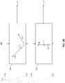
- FIG. 4B exemplary local prototypes for "side-only" channels are illustrated. Note that in other examples, local prototypes may be derived from a single channel, while in other examples they may be derived from two or more than two channels.
- a part of each of the input signals 412 is combined to create the center prototype.
- the local "side-only" prototypes are the remainder of each input signal 412 after contributing to the center channel. For example, referring to l o ( t ), if l ( t ) is smaller than r(t), the prototype is equal to zero. When l ( t ) is greater than r(t), the prototype has a length that is the difference in the lengths of the input signals 412, and the same direction as input l(t).
- FIG. 4C an exemplary local prototype for a "surround” channel is illustrated.
- "Surround” prototypes can be used for upmixing based on difference (antiphase) information.
- This local prototype is symmetric with the center channel local prototype. It is maximal when the input signals 412 are equal in level and out of phase, and it decreases as the level differences increase or the phase differences decrease.
- h cl Re S CL S LL
- h cr Re S CR S RR .
- upmixing outputs are generated by mixing both left and right input into each upmixer output.
- least squares is used to solve for two coefficients for each upmixer output: a left-input coefficient and a right-input coefficient.
- the output is generated by scaling each input with the corresponding coefficient and summing.
- Left-only and right-only signals are then computed by removing the components of the center and surround signals from the input signals, as introduced above. Note that in other examples, the left only and right only channels may be extracted directly rather that computing them as a remainder after subtraction of other extracted signals.
- a number of example of a local prototype systhesis, for example for a center channel are presented above. However, a variety of heuristics, physical gating schemes, and signal selection algorithms could be employed to create local prototypes.
- the prototype signals d ( t ), for example, as illustrated in FIG. 1 and FIG. 2 do not necessarily have to be calculated explicitly.
- formulas are determined to compute the auto and cross power spectra, or other characterizations of prototype signals, that are then used in determining weights w k 217 used in an estimator 210 without actually forming the signal d(t) 209, while still yielding the same or substantially same result as would have been obtained through explicit computation of the prototype.
- other forms of estimator do not necessarily use weighted input signals to form the estimated signals.
- Some estimators do not necessarily make use of explicitly formed prototype signals and rather use signal or data characterizing the prototypes of the target signal (e.g., using values representing statistical properties, such as auto- or cross correlation estimate, moments, etc., of the prototype) in such a way that the output of the estimator is the estimate according to the particular metric used by the estimator (e.g., a least squares error metric).
- the estimation approach can be understood as a subspace projection, which the subspace is defined by the set of input signals used as the basis for the output.
- the prototypes themselves are a linear function of the input signals, but may be restricted to a different subspace defined by a different subset of input signals than is used in the estimations phase.
- the prototype signals are determined using different representations than are used in the estimation.
- the prototypes may be determined using different or no component decompositions that are not the same as the component decomposition used in the estimation phase.
- local prototypes may not necessarily be strictly limited to prototypes computed from input signals in a single component (e.g., frequency band) and a single time period (e.g., a single window of the input analysis). For instance, there may be limited used of nearby components (e.g., components that are perceptually near in time and/or frequency) while still providing relatively more locality of prototype synthesis than the locality of the estimation process.
- a single component e.g., frequency band
- time period e.g., a single window of the input analysis
- the smoothing introduced by the windowing of the time data could be further extended to masking based time-frequency smoothing or non linear, time invariant (LTI) smoothing.
- coefficient estimation rules could be modified to enforce a constant power constraint. For instance, rather than computing residual "side-only" signals, multiple prototypes can be simultaneously estimated while preserving a total power constraints such that the total left and right signals are maintained over the sum of output channels.
- the input space may be rotated. Such a rotation could produce cleaner left only and right only spatial decompositions. For example, left-plus-right and left-minus-right could be used as input signals (input space rotated 45 degrees). More generally, the input signals may be subject to a transformation, for instance, a linear transformation, prior to prototype synthesis and/or output estimation.
- the method described in this application can be applied in a variety of applications where input signals need to be spatially separated in a low latency and low artifact manner.
- the method could be applied to stereo systems such as home theater surround sound systems or automobile surround sound systems.
- stereo systems such as home theater surround sound systems or automobile surround sound systems.
- the two channel stereo signals from a compact disc player could be spatially separated to a number of channels in an automobile.
- the described method could also be used in telecommunication applications such as telephone headsets.
- the method could be used to null unwanted ambient sound from the microphone input of a wireless headset.
- Examples of the approaches described above may be implemented in software, in hardware, or in a combination of hardware and software.
- the software may include a computer readable medium (e.g., disk or solid state memory) that holds instructions for causing a computer processor (e.g., a general purpose processor, digital signal processor, tec.) to perform the steps described above.
- a computer processor e.g., a general purpose processor, digital signal processor, tec.
- the approaches are embodied in a sound processor device which is suitable (e.g., configurable) for integration into one or more types of systems (e.g., home audio, headset, etc.)
Landscapes
- Physics & Mathematics (AREA)
- Engineering & Computer Science (AREA)
- Algebra (AREA)
- General Physics & Mathematics (AREA)
- Mathematical Analysis (AREA)
- Mathematical Optimization (AREA)
- Mathematical Physics (AREA)
- Pure & Applied Mathematics (AREA)
- Theoretical Computer Science (AREA)
- Acoustics & Sound (AREA)
- Signal Processing (AREA)
- Circuit For Audible Band Transducer (AREA)
Description
- This application is a continuation-in-part (CIP) of the following application:
- ■ U.S. Application Serial No.
12/909,569, filed on October 21, 2011 - This application is related to, but does not claim the benefit of the filing dates of, the following applications:
- ■
U.S. Patent No. 7,630,500 , titled "Spatial Disassembly Process," issued on December 8, 2009; and - ■
U.S. Patent Pub. 2009/0262969 , titled "Hearing Assistance Apparatus," published on October 22, 2009. - ■
U.S. Patent Pub. 2008/0317260 , titled "Sound Discrimination Method and Apparatus," published on December 25, 2008. - This invention relates to estimation of synthetic audio prototypes.
- In the field of audio signal processing, the term "upmixing" generally refers to the process of undoing "downmixing", which is the addition of many source signals into fewer audio channels. Downmixing can be a natural acoustic process, or a studio combination. As an example, upmixing can involve producing a number of spatially separated audio channels from a multichannel source.
- The simplest upmixer takes in a stereo pair of audio signals and generates a single output representing the information common to both channels, which is usually referred to as the center channel. A slightly more complex upmixer might generate three channels, representing the center channel and the "not center" components of the left and right inputs. More complex upmixers attempt to separate one or more center channels, two "side-only" channels of panned content, and one or more "surround" channels of uncorrelated or out of phase content.
- One method of upmixing is performed in the time domain by creating weighted (sometimes negative) combinations of stereo input channels. This method can render a single source in a desired location, but it may not allow multiple simultaneous sources to be isolated. For example, a time domain upmixer operating on stereo content that is dominated by common (center) content will mix panned and poorly correlated content into the center output channel even though this weaker content belongs in other channels.
- A number of stereo upmixing algorithms are commercially available, including Dolby Pro Logic II (and variants), Lexicon's Logic 7 and DTS Neo:6, Bose'sVideostage, Audio Stage, Centerpoint, and Centerpoint II.
- There is a need to perform upmixing in a manner that accurately renders spatially separated audio channels from a multichannel source in a manner that reduces sonic artifacts and has low processing latency.
-
WO 2008/155708 ,US 2009/110203 ,US 2008/152155 andUS 2006/045294 disclose prior art methods and systems in the audio signal processing field. - The present invention relates to a method for forming one audio output signal from a plurality of audio input signals, as recited in
claim 1. Advantageous embodiments are set out in dependent claims of the appended set of claims. -
-
FIG. 1 is a block diagram of a system configured for linear estimation of synthetic prototypes. -
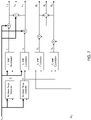
FIG. 2 is a block diagram of the decomposition of signals into components and estimation of a synthetic prototype for a representative component. -
FIG. 3A shows a time-component representation for a prototype. -
FIG. 3B is a detailed view of a single tile of the time-component representation. -
FIG. 4A is a block diagram showing an exemplary center channel synthetic prototype di (t). -
FIG. 4B is a block diagram showing two exemplary "side-only" synthetic prototypes di (t). -
FIG. 4C is a block diagram showing an exemplary surround channel synthetic prototype di (t). -
FIG. 5 is a block diagram of an alternative configuration of the synthetic processing module. -
FIG. 6 is a block diagram of a system configured to determine upmixing coefficient h. -
FIG. 7 is a block diagram illustrating how six upmixing channels can be determined by using two local prototypes. -
FIG. 8 is a block diagram of a system including a prototype generator that utilizes multiple past inputs and outputs. -
FIG. 9 is a two-microphone array receiving a source signal. -
FIG. 10 is a two-microphone array receiving a source signal and a noise signal. -
FIG. 11 is a graph of measured average Signal to Noise Ratio Gain and Preserved Signal Ratios of an MVDR design versus the a time-frequency masking scheme. -
FIG. 12 is a graph of average target and noise signal power. -
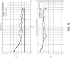
FIG. 13 is a graph of Signal to Noise Ratio Gain and Preserved Signal Ratios. -
FIG. 14 is a graph of Signal to Noise Ratio Gain and Preserved Signal Ratios. -
FIG. 15 is a graph of Signal to Noise Ratio Gain and Preserved Signal Ratios. - Referring to
FIG. 1 , an example of a system that makes use of estimation of synthetic prototypes is anupmixing system 100 that includes anupmix module 104, which accepts input signals 112 s 1(t),...,sN (t) and outputs an upmixed signal d̂(t). As an example, input time signals s 1(t) and s 2(t) represent left and right input signals, and d̂(t) represents a derived center channel. Theupmix module 104 forms the upmixed signal d̂(t) as a combination of the input signals s 1(t),...,sN (t) 112, for instance as a (time varying) linear combination of the input signals. Generally, the upmixed signal d̂(t) is formed by anestimator 110 as a linear estimate of the prototype signal d(t) 109, which is formed from the input signals by aprototype generator 108, generally by a non-linear technique. In some examples, the estimate is formed as a linear (e.g., frequency weighted) combination of the input signals that best approximates the prototype signal in a minimum mean-squared error sense. This linear estimate d̂(t) is generally based on agenerative model 102 for the set ofinput signals 112 as being formed as a combination of an obscured target signal d̂(t) andnoise components 114 each associated with one of theinput signal 112. - In the
system 100 shown inFIG. 1 , a syntheticprototype generation module 108 forms the prototype d(t) 109 as nonlinear transformations of the set ofinput signals 112. It should be recognized that the prototype can also be formed using linear techniques, as an example, with the prototype being formed from a different subset of the input signals than is used to estimate the output signal from the prototype. For certain types of prototype generation, the prototype may include degradation and/or artifacts that would produce low quality audio output if presented directly to a listener without passing through thelinear estimator 110. As introduced above, in some examples, the prototype d(t) is associated with a desired upmixing of input signals. In other examples, the prototype is formed for other purposes, for example, based on an identification of a desired signal in the presence of interference. - In some embodiments, the process of forming the prototype signal is more localized in time and/or frequency than is the estimation process, which may introduce a degree of smoothness that can compensate for unpleasant characteristics in the prototype signal resulting from the localized processing. On the other hand, the local nature of the prototype generation provides a degree of flexibility and control that enables forms of processing (e.g., upmixing) that are otherwise unattainable.
- In some implementations, the
upmixing module 104 of theupmixing system 100 illustrated inFIG. 1 is implemented by breaking eachinput signal 112 into components (e.g., frequency bands) and processing each component individually. For example, in the case of orthogonal components, thelinear estimator 110 can be implemented by independently forming an estimate of each orthogonal component, and then synthesizing the output signal from the estimated components. It should be understood that although the description below focuses on components formed as frequency bands of the input signals, other decompositions into orthogonal or substantially independent components may be equivalently used. Such alternative decomposition may include Wavelet transform of the input signals, non-uniform (e.g., psychoacoustic critical bands; octaves) filter banks, perceptual component decomposition, quadrature mirror filterbanks, statistical (e.g., principal components) based decompositions, etc. - Referring to
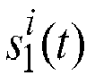
FIG. 2 , one embodiment of anupmixing module 104 is configured to process decompositions of the input signals (in this example two input signals) in a manner similar to that described inU.S. Patent 7,630,500 , titled "Spatial Disassembly Process,". Each of the input signals 112 is transformed into a multiple component representation withindividual components 212. For instance, the input signal s 1(t) is decomposed into a set of components
component analyzer 220 is a discrete Fourier transform (DFT) analysis filter bank that transforms the input signals into frequency components. In some examples, the frequency components are outputs of zero-phase filters, each with an equal bandwidth (e.g., 125Hz). - The output signal d̂(t) is reconstructed from a set of components d̂i (t) using a
reconstruction module 230. The component analyzers 220 and thereconstruction module 230 are such that if the components are passed through without modification, the originally analyzed signal is essentially (i.e., not necessarily perfectly) reproduced at the output of thereconstruction module 230. - In some embodiments, the
component analyzer 220 windows the input signals 112 into time blocks of equal size, which may be indexed by n. The blocks may overlap (i.e., part of the data of one block may also be contained in another block), such that each window is shifted in time by a "hop size" τ. As an example, a windowing function (e.g., square root Hanning window) may be applied to each block for the purpose of improving the resulting component representations 222. Following applying the windowing function to the blocks, thecomponent analyzer 220 may zero pad each block of the input signals 112 and then decompose each zero padded block into their respective component representations. In some embodiments, thecomponents 212 form base band signals, each modulated by a center frequency (i.e., by a complex exponential) of the respective center frequencies of the filter bands. Furthermore eachcomponent 212 may be downsampled and processed at a lower sampling rate sufficient for the bandwidth of the filter bands. For example, the output of a DFT filter bank band-pass filter with a 125Hz bandwidth may be sampled at 250Hz without violating the Nyquist criterion. - In some examples, the input signals are sampled at 44.1 KHz, and shifted into frames of length 23.2 ms., or 1024 samples, that are selected at a frame hop period of τ = 11.6 ms, or 512 samples. Each frame is multiplicatively windowed by a window function of sin(π·t) / τ, where t=0 indexes the beginning of the frame. The windowed frame forms the input to a 1024_point FFT. Each frequency component is formed from one output of the FFT. (Other windows may be chosen that are shorter of longer than the input length of the FFT. If the input window is shorter than the FFT, the data can be zero-extended to fit the FFT; if the input window is longer than the FFT, the data can be time-aliased.)
- In
FIG. 2 , the windowing of the input signals, and the subsequent overlap adding of the output signals is not illustrated. Therefore, the figure should be understood as explicitly illustrating the processing of a single analysis window. More precisely, given the continuous input signal sk(t), for the n th analysis window, a windowed signal s k,[n](t) = sk (t)w(t- nτ) is formed, where the window may be defined as w(t) = sin(π·t) / τ These windowed signals are shown without subscripts [n] inFIG. 2 . The components of a signal are then defined to decompose each signal as
- As introduced above, one approach to synthesis of prototype signals is on a component-by-component basis, and in particular in a component-local basis such that each component for each window period is processed separately to form one or more prototypes for that local component.
- In
FIG. 2 , acomponent upmixer 206 processes a single pair of input components,

local prototype generator 208 which determines a prototype signal component di (t) (typically at the downsampled rate) from the input components

linear estimator 210, then estimates the output component d̂i (t). - The
local prototype generator 208 can make use of synthesis techniques that offer the possibility to perform a wide range of transforms that might not otherwise be possible by using linear processing techniques alone. For example, upmixing, modification of room acoustics, and signal selection (e.g., for telephones and hearing aids) can all be accomplished using this class of synthetic processing techniques. - In some embodiments, the local prototype signal is derived based on knowledge, or an assumption, about the characteristics of the desired signal and undesired signals, as observed in the input signal space. For instance, the local prototype generator selects inputs that display the characteristics of the desired signal and inhibits inputs that do not display the desired characteristics. In this context, selection means passing with some pre-defined maximum gain, example unity, and in the limit, inhibition means passing with zero gain. Preferred selection functions may have a binary characteristic (pass region with unity gain, reject region with zero gain) or a gentle transition between passing signals with desired characteristics and rejecting signals with undesired characteristics. The selection function may include a linear combination of linearly modified inputs, one or more nonlinearly gated inputs, multiplicative combinations of inputs (of any order) and other nonlinear functions of the inputs.
- In some embodiments, the
synthetic prototype generator 208 generates what are effectively instantaneous (i.e., temporally local) "guesses" of signal desired at the output, without necessarily considering whether a sequence of such guesses would directly synthesize an artifact-free signal. - In some examples, approaches described in
U.S. Patent 7,630,500 , that are used to compute components of an output signal are used in the present approaches to compute components of a prototype signal, which are then subject to further processing. Note that in such examples, the present approaches may differ from those described in the referenced patent in characteristics such as the time and/or frequency extent of components. For instance, in the present approach, the window "hop rate" may be higher, resulting a more temporally local synthesis of prototypes, and in some synthesis approaches, such a higher hop rate might result in more artifacts if the approaches described in the referenced patent were used directly. - Referring to
FIG. 4A , one exemplary multiple input local prototype di (t) generator 408 (an instance of thenon-linear prototype generator 208 shown inFIG. 2 ) for a center channel is illustrated in the complex plane for a single time value. A formula, which is applied independently for each component, defines this particular local prototype:
U.S. Patent 7,630,500 at equation (16), in which
- Note that the input signals 412,

inputs 412, the one with the larger magnitude is scaled by a real coefficient to match the length of the smaller, and then the average of the two is taken. This local prototype signal has a selection characteristic such that its output is largest in magnitude when the twoinputs 412 are in phase and equal in level, and it decreases as the level and phase differences between the signals increase. It is zero for "hard-panned" and phase-reversed left and right signals. Its phase is the average of the phase of the two input signals. Thus the vector gating function can generate a signal that has a different phase than either of the original signals, even though the components of the vector gating factor are real-valued. - Referring to
FIG. 5 , another example of a prototype generation module 508 (which is another instance of theprototype generator 208 shown inFIG. 2 ) includes agating function 524 and ascaler 526. Thegating function 524 module accepts the input signals 512 and uses them to determine a gating factor gi , which is kept constant during the analysis interval corresponding to one windowing of the input signal. Thegating function module 524 may be switched between 0 and 1 based on the input signals 512. Alternatively, thegating function module 524 may implement a smooth slope, where the gating is adjusted between 0 and 1 based on the input signals 512 and/or their history over many analysis windows. One of the input signals 512, for instance
scaler 526 to yield local prototype d(t) . This operation dynamically adjusts the amount ofinput signal 512 that is included in the output of the system. Because g is a function of s 1, d(t) is not a linear function of s 1, and is thus the local prototype is a non-linear modification of s 1 that has a dependency on s 2. Because the gating factor is real only, the local prototype, d, has the same phase as s 1; only its magnitude is modified. Note that the gating factor is determined on a component-by-component basis, with the gating factor for each band being adjusted from analysis window to analysis window. - One exemplary use of a gating function is for processing input from a telephone headset. The headset may include two microphones configured to be spaced apart from one another and substantially co-linear with the primary direction of acoustic propagation of the speaker's voice. The microphones provide the input signals 512 to the
prototype generation module 508. Thegating function module 524 analyzes the input signals 512 by, for example, observing the phase difference between the two microphones. Based on the observed difference, thegating function 524 generates a gating factor gi for each frequency component i. For example, the gating factor gi may be 0 when the phase at both microphones is equal, indicating that the recorded sound is not the speaker's voice and instead an extraneous sound from the environment. Alternatively, when the phase between the input signals 512 corresponds to the acoustic propagation delay between the microphones, the gating factor may be 1. - In general, a variety of prototype synthesis approaches may be formulated as a gating of the input signals in which the gating is according to coefficients that range from 0 to 1, which can be expressed in vector-matrix form as:

- In another example, the gating function is configured for use in a hearing assistance device in a manner similar to that described in
U.S. Patent Pub. 2009/0262969 , titled "Hearing Assistance Apparatus", which is incorporated herein by reference. In such a configuration, the gating function is configured to provide more emphasis to a sound source that a user is facing than a sound source that a user is not facing. - In another example, the gating function is configured for use in a sound discrimination application in which the prototype is determined in a manner similar to the way that output components are determined in
U.S. Patent Pub. 2008/0317260 , titled "Sound Discrimination Method and Apparatus," which is incorporated herein by reference. For example, the output of the multiplier (42), which is the product of an input and a gain (40) (i.e., gating term) in the referenced publication, is applied as a prototype in the present approaches. - Referring back to
FIG. 1 , theestimator 110 is configured to determine the output d̂(t) that best matches a prototype d(t). In some embodiments, theestimator 110 is a linear estimator that matches d̂(t) in a least squares sense. Referring back toFIG. 2 , for at least some forms ofestimator 110, this estimate may be performed on a component by component basis because generally, the errors in each component are uncorrelated resulting from the orthogonality of the components, and therefore each component can be estimated separately. Thecomponent estimator 210 forms the estimate d̂i(t) as a weighted combination
squares weight estimator 216 to form lowest error estimate based on auto and cross power spectra of the input signals s 1(t) and s 2 (t) . - The computation implemented in some examples of the estimation module may be understood by considering a desired (complex) signal d̂(t) and a (complex) input signal x(t) with the goal being to find the real coefficient h such that |d(t) - hx(t)|2 is minimized. The coefficient that minimizes this error can be expressed as

- where the exponent ∗ represents a complex conjugate and E{ } represents an average or expectation over time. Note that numerically, the computation of h can be unstable if E(x 2 (t)) is small, so numerically, the estimate is adjusted adding a small value to the denominator as

- As applied to the windowed analysis illustrated in
FIG. 2 , (using the notation [n] to refer to the nth window) given a windowed input signal x [n](t) (i.e., the nth window of an input signal x(t)), one of the sk (t), and the corresponding prototype d [n](t), a local estimate of the auto and cross correlations within that window is formed as
- In order to obtain robust estimates of the auto- and cross-correlation coefficients, a time averaging or filtering over multiple time windows may be used. For example, one form of filter is a decaying time average computed over past windows:

- Referring to
FIG. 6 , oneembodiment 700 of the least squaresweight estimation module 216 is illustrated for the case of estimating a weight h for forming the prototype based on a single component. The component of the input is identified as X in the figure (e.g., a component si (t) downsampled to a single sample per window), and the prototype component is identified as D in the figure.FIG. 6 represents a discrete time filtering approach that is updated once every window period. In particular, SDX is calculated along the top path by computing thecomplex conjugate 750 of X, multiplying 752 the complex conjugate of X by D, and then low-pass filtering 754 that product along the time dimension. The real part of SDX is then extracted. SXX is calculated along the bottom path by squaring themagnitude 760 of X and then low-pass filtering 762 the result along the time dimension. A small value ε is then added 764 to SXX to prevent division by zero. Finally, h is calculated by dividing 758 Re{ SDX } by SXX + ∈. - The computation implemented by the estimation module may be further understood by considering a desired signal d(t) formed as combination of two inputs x(t) and y(t) with the goal being to find the real coefficients h and g such that |d(t) - hx(t) - gy(t)|2 is minimized. Note that the using real coefficients is not necessary, and in alternative embodiments with complex coefficients, the formulas for the coefficient values are different (e.g., for complex coefficients, the Re( ) operation is dropped on all terms). In this case with real coefficients, the coefficients that minimize this error can be expressed as

- As introduced above, each of the auto- and cross-correlation terms are filtered over a range of windows and adjusted prior to computation.
- The matrix formulation shown above for two channels is readily modified for any number of input channels. For example, in the case of a vector of m prototypes d(t) and a vector of n input signals
x (t), a m by n matrix of weighting coefficients H may be computed to form the estimate using the vector-matrix formula

- S
DX = Re(E{d (t )x H (t)}) is a n by m matrix and - S
XX = Re(E{x (t)x H (t)}) is a n by n matrix anddH indicates the transpose of the complex conjugate, and the covariance terms are computed and filtered and adjusted on a component-wise basis as described above. -
FIG. 3A is agraphical representation 300 of a time-component representation 322 for all the input channels sk (t) and the one or more prototypes d(t). Eachtile 332 in therepresentation 300 is associated with one window index n and one component index i.FIG. 3B is a detailed view of asingle tile 332. In particularFIG. 3B shows that thetile 332 is created byfirst time windowing 380 each of the input signals 312. The time windowed section of eachinput signal 312 is then processed by acomponent decomposition module 220. For eachtile 332, an estimate of theauto 384 and cross 382 correlations of theinput channels 312, as well ascross correlations 382 of each of the inputs and each of the outputs is computed, and then filtered 386 over time and adjusted to preserve numerical stability. Then each of the weighting coefficients
- Note that in the description above, the smoothing of the correlation coefficients is performed over time. In some examples, the smoothing is also across components (e.g., frequency bands). Furthermore, the characteristics of the smoothing across components may not be equal, for example, with a larger frequency extent at higher frequencies than at lower frequencies.
- In the examples below, for simplicity of notation, the dependence on the time variable t is omitted. Note that for some selections of analysis period τ, only a single value is needed to represent the component, and therefore omitting the dependence on t can be considered as corresponding to a single (complex) value representing the analysis component. Also, in general, the weighting values are generally complex rather than real as is the case in certain examples presented above.
- As a first example, to summarize an approach presented above, a scalar prototype d can be estimated from n inputs x (i.e., an n column vector) by estimating a vector of n weights w (i.e., an n column vector) to satisfy:


- The resulting least squares estimate of d , d̂, has a smoothing effect on d which can be perceptually pleasing to a listener. This estimate of the desired prototype, d̂ = w T x = d + e (where the e term is the remaining least squares estimation error) retains the desired characteristics of d, but can be more perceptually pleasing than d alone. Furthermore, d̂ can better retain the desired behavior of d than a simply smoothed version of d.
- In the previous example, a short-time implementation of the least squares solution is optionally implemented by applying low pass filters (i.e., short time expectation operators and/or cross-frequency smoothing of the statistics) to the cross and auto statistics of the closed-form solution to w. While the previous example uses the short-time implementation of the least squares solution for smoothing a single desired prototype signal, it is noted that the short-time implementation of least squares can be extended and applied to a variety of other problems (e.g., dynamic filter coefficients) by adding constraints. In particular, it can be seen as a short-time implementation of a time-varying closed form least-squares solution. This time-varying closed form least-squares solution can be applied to a variety of other situations.
- In general, in the approaches described above, the prototype estimate for a frequency component i at a time frame n is assumed to depend on input signals at that same component and frame index, and possibly indirectly on other components and time frames by smoothing of the statistics used in estimation. More generally, a prototype dn at time frame n (or more precisely a prototype dn,i for frequency component i at time frame n ; but the dependence on i is omitted for simplicity of notation) depends on inputs xn ,···,x n-k+1 over a range of k time frames n - k +1,···,n, and each input xi can be a vector of values that includes other frequency components than that of the prototype being estimated.
- Referring to
FIG. 8 , in a second example asystem 800 receives an input signal xn where n is, for example, the nth frame of the input signal. In this example, theprototype generator 802 utilizes multiple past inputs of the input component xn or past prototype estimates y n-1···yn-k to determine the prototype signal component dn at time n. One example of aprototype generator 802 assumes dn is a weighted linear combination of past inputs and past outputs of the input component plus some estimation error, such that the prototype estimate d̂n has the form of an IIR filter, as follows:


- The prototype signal component dn is passed to a component based linear estimator 804 (e.g., a least squares estimator) which determines the vector, w , which minimizes the difference between the prototype signal component dn and w T z in a least squares sense as follows:


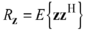
- Note that since z is a ( k + / + 1) column vector of input signals, R z is (k + / + 1) by (.. k+l+1 ..), so that for many input signals the inversion of R2 could be expensive.
- The output of the component based
linear estimator 804, w , is passed to a linear combination module 806 (e.g., an IIR filter) which forms the estimate d̂ as a combination of the past input and past output values of xn in the same manner as theprototype generator 802. However, thelinear combination module 806 uses the values included in the w vector in place of the b 0,b 1,···,bk and a 1,a 2,···,al values (i.e., replace b 0 with w b0, b 1 with w b1 , and so on). The output of thelinear combination module 806, d̂n , is the lowest error estimate of dn. - In some examples, it is desirable to estimate multiple prototype signals from multiple input signals such that the weights used for each prototype are constrained, for example to be the same for each prototype, but applied to different input signals. As one possible example, if each prototype is a different time frame (i.e., delay) of a particular signal component, then it may be desirable that the filtering of input components at different lags be time invariant. Another example is presented in Section 5.7 below.
- In general, let d be an N×1 vector of desired signals:
d = [d 0,d 1,···,d N-1]T and let w = [w 0,w 1,···,w P-1] T be a Px1 vector of coefficients used to linearly combine N separate Px1 vectors of input signals. The input signals combined using w may be different for each desired prototype signal in d. - Specifically, let there be a separate Px1 input vector x i (i = 0,1,···N -1) that corresponds to each desired signal or signal vector in

- An N×P input matrix, Z, can then be formed as:

- Then (noting that di = w T x i + e 0 = x i T w + e 0) the system of equations can be rewritten as


- The closed form solution which simultaneously minimizes the difference between each of the prototype signal components d and Zw in a least squares sense as follows:


- In the above example, each input value is effectively deemed to have the same importance in the determination of the prototype estimate by virtue of effectively minimizing the sum of the squares of the ei . However, in some examples it can be useful to allow certain inputs to count more or less than other inputs. This can be accomplished using a weighted least squares solution.
- The weighted least squares solution defines G as an N×N diagonal matrix of weights gi for each input xi :

- Including this matrix in the least squares solutions described above causes an error due to a higher weighted input constraint to cost more than an error due to a lower weighted input constraint. This biases the least squares solution toward constraints with greater weights. In some examples, the constraint weights vary with time and/or frequency and can be driven by other information within a system. In other examples, there can be situations within a given frequency band where one constraint should take precedence over another, and vice versa.
- The least squares solution including the matrix of weights W can be expressed as:

- In this example, the goal is to find the linear combination of two input channel signals at time index n, x 1,n and x 2,n , that is the best estimate d̂n of the desired signal dn at time nn . Thus,


- This result is commensurate with the example presented in section 5.1.
- This example differs from Example 1 in that instead of using two different channels as input, two different time segments of a single channel are used as input. The goal is find the linear combination of the current (at time n ) and previous (at time n -1) input signals, xn and x n-1, that is the best estimate d̂n of the desired signal dn at the current time n. Thus,


- Thus, Examples 1 and 2 illustrate that it is possible to solve for the local desired signal dn by taking inputs across both channels and/or time. The dimension P, however, becomes greater than two and inverting a P×P matrix Z H Z can be expensive. Note that additional desired signals (which correspond to additional input constraints, i.e. the dimension N ) can be used without increasing the size of the PxP matrix inversion.
- In some examples, least squares smoothing is applied to a microphone array. The raw signals from the microphones in the array are used to estimate a desired source signal component at specific points in time and frequency. The goal is to determine a linear combination of the microphone signals which best approximates an instantaneous desired signal at the specific points in time and frequency. Such an application can be thought of as an extension of the application described in Example 1 above.
- As is described more fully below, the least squares solution may not only provide the desired smoothing behavior to the desired signal, but can also produce coefficients which provide cancellation when the coefficients solved are complex valued.
- Referring to
FIG. 9 , asource 1002 at an ideal or known source location produces a source signal (e.g., an audio signal) which propagates through the air to eachmicrophone 1004 of amicrophone array 1006 that includes in this example two microphones, M1 and M2. As the source signal propagates from thesource 1002 to eachmicrophone 1004, it is assumed to pass through a linear transfer function Hdp where p is the pth microphone 1004 in themicrophone array 1006. In the discussion below, the transfer function of a particular signal component (e.g., frequency band) is referred to as hdp . - If the geometry of the desired
source 1002 location with respect to amicrophone array 1006 is known, the set of transfer functions, between theideal source location 1002 and the two microphones in themicrophone array 1006 can be expressed as
- One example of such a situation is in the case of an ear-mounted microphone array in which the location of the mouth is known (at least approximately) relative to the microphones, and therefore the transfer function may be predetermined or estimated during use.
- One approach, which is not discussed further below, to processing an array of microphone signals where the transfer functions Hdp are known could be to first estimate the source signal s and the apply this signal to prototype estimation procedures as described above.
- Another preferable approach is to form the prototype estimates from the separate input signals in such a way that the weighting of the input signals approximately (but not necessarily) matches the known transfer functions from the ideal source location. In this way, a signal arriving from the ideal source location is generally passed without modification.
- One way to accomplish this is to augment the prototype dn with a unit prototype d = [dn ,1]T. The unit prototype is derived from the distortionless response constraint which is used in obtaining the more commonly known Minimum Variance Distortionless Response (MVDR) solution as follows:

- To determine the weighting vector such that the weighted input signals approximately match the known transfer functions from the source, s is substituted for d in the above equation as follows:


- In the context of the general least squares solution, the prototype and input matrices can then be expressed as:


- Note that the above solution combines a time invariant constraint with a time-varying solution. Thus, the additional constraint can be used to help restrain the instantaneous solution for w based on estimating dn alone from substantially harming any source signal that originated from the ideal source location. Note, however, that this is not an absolute constraint as is the case for the MVDR solution (which strictly forbids any distortion in the target source direction).
- As is described above, in some examples it is desirable to have certain prototypes in the vector of prototypes, d, to have more or less effect on the estimated signal than other prototypes. This can be accomplished by including a weighting vector, G, in the solution for w. Thus the weighted solution for the example shown in
FIG. 9 is as follows:
- Referring to
FIG. 10 , the above example can be extended to include an additional constraint such that the instantaneous coefficients w produce a null in a particular direction with respect to themicrophone array 1106. For example, the direction can be expressed as a transfer function Hnp (where p is the pth microphone) between a noise (or otherwise not desired) source,N 1108 at an ideal or known noise location and theP microphones 1104 in themicrophone array 1106. For the discussion below, the transfer function of a signal component (e.g., a frequency band) is referred to as hnp. For the example ofFIG. 10 , the desired prototype vector and input matrix (for the 2 microphone elements case) can be expressed as follows:

- The weighted solution for this example produces a tendency towards a null (i.e., an attenuation) approximately in the direction of the noise source while preserving the source signal.
- While the two examples described above each involve the use of two microphones, the number of microphones can be some other number P which is greater than two. In this general case, the inputs can be expressed as:


- Furthermore, while the examples above describe prototypes which apply to nulling and beamforming, it is noted that any other arbitrary prototypes can be used.
- In another example, a two element microphone array produces raw input signals x 1 and x 2. By observing differences in the raw input signals, an instantaneous estimate of the desired signal component in each microphone, d 1 and d 2 can be obtained. These local estimates of the desired signal can be used to obtain local estimates of the noise signal from each microphone signal as follows:


- In one of the examples above, the application of least squares smoothing to a microphone array was used to clean up an estimate of the desired signal. The goal of the above example was to determine a linear combination of the microphone inputs which best approximated a desired signal estimate. In this example an additional goal is to determine, at a given time-frequency point, what is the linear combination of the input signals that would best cancel a local estimate of the noise signals, while still attempting to preserve the target signal. Using the general least squares solution, the problem can be expressed as:


- Here, the top row in Z is again the transfer functions from the desired source to the array, and the desired array response in that direction is 1, while the desired response to the instantaneous noise estimate is some small signal a.

- In another example, Example 4a is extended to include the original input constraint. Thus, the input matrix and desired vector are expressed as:


- Given that the solution for w is computed for each frequency component, the constraint weights can vary as a function of time and frequency (W = W(t,f)). In some examples, it is advantageous to give more weight to certain constraints within specific frequency ranges at certain times.
- It is noted that as the number of constraints being included increases, the overall formulation of a weighted, constrained least squares smoothing structure can in general be seen as an implementation strategy for incorporating multiple desired behaviors with narrow time and frequency resolution. Furthermore, in some examples it may be impossible to simultaneously obtain all of the desired behaviors due to limited degrees of freedom or conflicting requirements. However, this formulation allows the desired behaviors to be dynamically emphasized (smoothly switching or blending between constraints), while the individual constraints are smoothed in a desirable way.
- In another example, both a distortionless response and noise cancellation are desired. The input matrix and desired prototype vector are expressed as:


- where a = 0 or some small signal/value. In this example, the emphasis of each constraint depends on a time and/or frequency varying value. For example, a weight matrix can be defined as:
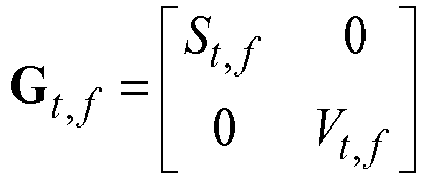
- Where, S t,f may function to emphasize the distortionless response constraint when the estimated target signal is present (or significant) and focus less on the distortionless response constraint when the estimated target signal is not present (or insignificant). One example of St,f is |dn |2 which is an instantaneous estimate of the target signal energy. Placing |dn |2 in the weight matrix has the effect of emphasizing the distortionless response (DR) constraint when the energy of the target signal is high. Therefore, when the target signal is absent the solution focuses more on satisfying the noise cancellation constraint. Vt,f is an arbitrary weight function on the noise cancellation constraint which may vary with time or frequency. It is noted that the dynamic weighting of constraints shown above is only one example and in general, any arbitrary function (e.g., inter-microphone coherence) can be used for dynamic weighting.
- In one example, two input signals are available, U and S ( which like all previous examples may be multichannel time or frequency domain signals). In this example, both U and S include the same desired signal but different noise signals (i.e. U = s + Nu , and S = s + Ns ). Since both the desired signal and both noise signals may be time-varying and nonstationary, it can be useful to find a local time-frequency combination of U and S (i.e. wUU + wsS ) which includes the smallest possible noise contribution while preserving the wanted signal component that is present in both.
- In this example, the desired prototypes, inputs, and weights can be expressed as:



- In another example, the weights described in Example 5a are strictly enforced to have a blender relationship where the output signal Y = αkU + (1- αk )S is produced by the system. The blending factor , αk , can be dynamically determined as follows:

- In this example, the cost function collapses to a scalar error function such that the derivate with respect to α can be computed. However, as in the examples above, lowpass filters are used to obtain short-time expectation operations (i.e., E{ } ), as in least squares smoothing, to obtain fast, local estimates of αk.
- Time-frequency masking or gating schemes have the potential to outperform more well known LTI methods such as the MVDR solution under certain conditions. However, in very low SNR conditions where the target signal is seldom the dominant source, a time-frequency masking scheme tends to suppress too much of the desired signal, and may not necessarily improve the signal-to-noise ratio as well as a static spatial filter (i.e. MVDR). For a given noise environment, the optimal LTI solution results in a constant improvement in signal to noise independent of the environmental signal-to-interference ratio.
FIG. 11 compares the measured average SNR Gain and Preserved Signal Ratios (PSR) of an MVDR design versus the current time-frequency masking scheme which uses complex least squares smoothing. A negative PSR in the bottom half ofFIG. 11 represents on average how much of the target signal was lost (in dB) as a result of the array processing. This particular scenario includes a target speech signal in reverberated babble mixed to an overall rms SNR of -6dB. The average target and noise signal power spectra for this experiment are shown inFigure 12 . Note that above 1.5kHz where the local SNR is roughly 0 dB, the time-frequency masking scheme has minimal target signal loss but still a few dB of SNR gain compared to the static MVDR design. In the 400-600Hz range where the target has significant energy on average, but the SNR is poor (~-6dB), the time-frequency masking scheme provides up to 8dB of SNR Gain but at the cost of more target signal loss. Below 150Hz where the local SNR is very poor, the MVDR solution does a much better job at removing the noise compared to the time-frequency masker. - By applying additional constraints to the weighted least squares solution, as in Example 4b, it is possible to tradeoff different performance characteristics, even in the frequency ranges where each is most relevant. Furthermore, the audio quality benefits of the original least squares smoothing approach can be mostly preserved while adding this flexibility. In the following example, the constrained least squares approach was used to obtain a single solution that combines some of the strengths of both the MVDR and time-frequency masking methods. The desired vector and input matrix used were the following:


FIG. 13 . - Notice that the SNR Gain benefits of the time-frequency masker are mostly preserved while also improving the SNR gain below 200 Hz to equal that of the MVDR solution. The PSR of the constrained least squares approach is only slightly improved in this case, but is at least no worse than using the time-frequency masker alone.
FIG. 14 demonstrates the results using a different set of weight functions, when the distortionless response constraint is given even more emphasis at some frequencies. The SNR Gain is mostly as good as or better than the MVDR solution, but the PSR is improved over the previous example. -
FIG. 15 demonstrates the behavior when only the first two constraints are used (i.e., unity response and cancellation) with the unit response constraint configured to dominate via the weighting matrix. The performance clearly approaches the static MVDR solution. Thus, including these additional weighted constraints in the least squares smoothing solution can provide multiple benefits. It continues to provide the desired smoothing behavior of the original least squares approach. Furthermore, for the microphone array application using time-frequency masking, it allows the array processor to trade-off different desired behaviors (via the weight functions) to produce a more optimal solution. Furthermore, because the addition of multiple constraints does not increase the size of the matrix inversion in the least squares solution, the additional processing requirements might not be considerable. - Because the component decomposition module 220 (e.g. a DFT filter bank) has linear phase, the single channel upmixing outputs have the same phase and can be recombined without phase interaction, to effect various degrees of signal separation.
- The component reconstruction is implemented in a
component reconstruction module 230. Thecomponent reconstruction module 230 performs the inverse operation of thecomponent decomposition module 220, creating a spatially separated time signal from a number of components 222. - In
Section 3, with the input signals s 1(t) and s 2(t) corresponding to left, l(t), and right, r(t), signals, respectively, the prototype d̂(t) is suitable for a center channel, c(t). In one example, a similar approach may be applied to determine prototype signals for "left only", lo(t), and "right only", ro (t), signals. Referring toFIG. 4B , exemplary local prototypes for "side-only" channels are illustrated. Note that in other examples, local prototypes may be derived from a single channel, while in other examples they may be derived from two or more than two channels. - The following formulas define one form of such exemplary prototypes:
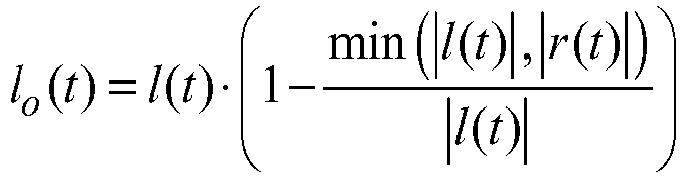

input signal 412 after contributing to the center channel. For example, referring to lo (t), if l(t) is smaller than r(t), the prototype is equal to zero. When l(t) is greater than r(t), the prototype has a length that is the difference in the lengths of the input signals 412, and the same direction as input l(t). - Referring to
FIG. 4C , an exemplary local prototype for a "surround" channel is illustrated. "Surround" prototypes can be used for upmixing based on difference (antiphase) information. The following formula defines the "surround" channel local prototype:
- Given prototype signals, for example, as described above, examples of approaches for estimating those prototype signals may differ in terms of the inputs combined to form the estimate. For instance, as illustrated in
FIG. 7 , the prototype d(t), referred to here as c(t) as the center channel prototype can yield two estimates, l̂c (t) and r̂c (t), each of which is formed as a weighting of a single input as


- In this example, there are four upmixed channels as defined above:
l̂c (t), r̂c (t), l̂s (t), and r̂s (t).
Two additional channels are calculated as the residual left and right signals after removing the single-channel center and surround components:

- In another example, upmixing outputs are generated by mixing both left and right input into each upmixer output. In this case, least squares is used to solve for two coefficients for each upmixer output: a left-input coefficient and a right-input coefficient. The output is generated by scaling each input with the corresponding coefficient and summing.
- In this example, if the center and surround channels are approximated as:


- Left-only and right-only signals are then computed by removing the components of the center and surround signals from the input signals, as introduced above. Note that in other examples, the left only and right only channels may be extracted directly rather that computing them as a remainder after subtraction of other extracted signals.
- A number of example of a local prototype systhesis, for example for a center channel are presented above. However, a variety of heuristics, physical gating schemes, and signal selection algorithms could be employed to create local prototypes.
- It should be understood that the prototype signals d(t), for example, as illustrated in
FIG. 1 andFIG. 2 , do not necessarily have to be calculated explicitly. In some examples, formulas are determined to compute the auto and cross power spectra, or other characterizations of prototype signals, that are then used in determining weights wk 217 used in anestimator 210 without actually forming the signal d(t) 209, while still yielding the same or substantially same result as would have been obtained through explicit computation of the prototype. Similarly, other forms of estimator do not necessarily use weighted input signals to form the estimated signals. Some estimators do not necessarily make use of explicitly formed prototype signals and rather use signal or data characterizing the prototypes of the target signal (e.g., using values representing statistical properties, such as auto- or cross correlation estimate, moments, etc., of the prototype) in such a way that the output of the estimator is the estimate according to the particular metric used by the estimator (e.g., a least squares error metric). - It should also be understood that in some examples, the estimation approach can be understood as a subspace projection, which the subspace is defined by the set of input signals used as the basis for the output. In some examples, the prototypes themselves are a linear function of the input signals, but may be restricted to a different subspace defined by a different subset of input signals than is used in the estimations phase.
- In some examples, the prototype signals are determined using different representations than are used in the estimation. For example, the prototypes may be determined using different or no component decompositions that are not the same as the component decomposition used in the estimation phase.
- It should also be understood that "local" prototypes may not necessarily be strictly limited to prototypes computed from input signals in a single component (e.g., frequency band) and a single time period (e.g., a single window of the input analysis). For instance, there may be limited used of nearby components (e.g., components that are perceptually near in time and/or frequency) while still providing relatively more locality of prototype synthesis than the locality of the estimation process.
- The smoothing introduced by the windowing of the time data could be further extended to masking based time-frequency smoothing or non linear, time invariant (LTI) smoothing.
- The coefficient estimation rules could be modified to enforce a constant power constraint. For instance, rather than computing residual "side-only" signals, multiple prototypes can be simultaneously estimated while preserving a total power constraints such that the total left and right signals are maintained over the sum of output channels.
- Given a stereo pair of input signals, L and R, the input space may be rotated. Such a rotation could produce cleaner left only and right only spatial decompositions. For example, left-plus-right and left-minus-right could be used as input signals (input space rotated 45 degrees). More generally, the input signals may be subject to a transformation, for instance, a linear transformation, prior to prototype synthesis and/or output estimation.
- The method described in this application can be applied in a variety of applications where input signals need to be spatially separated in a low latency and low artifact manner.
- The method could be applied to stereo systems such as home theater surround sound systems or automobile surround sound systems. For instance, the two channel stereo signals from a compact disc player could be spatially separated to a number of channels in an automobile.
- The described method could also be used in telecommunication applications such as telephone headsets. For example, the method could be used to null unwanted ambient sound from the microphone input of a wireless headset.
- Examples of the approaches described above may be implemented in software, in hardware, or in a combination of hardware and software. The software may include a computer readable medium (e.g., disk or solid state memory) that holds instructions for causing a computer processor (e.g., a general purpose processor, digital signal processor, tec.) to perform the steps described above. In some examples, the approaches are embodied in a sound processor device which is suitable (e.g., configurable) for integration into one or more types of systems (e.g., home audio, headset, etc.)
- It is to be understood that the foregoing description is intended to illustrate and not to limit the scope of the invention, which is defined by the scope of the appended claims.
Claims (11)
- A method for forming one audio output signal (114) from a plurality of audio input signals (112) comprising:synthesizing a prototype signal, wherein the synthesis of the prototype signal includes a non-linear function of the input signals, andforming one output signal, including forming the output signal as a linear estimate of the prototype signal, the linear estimate is formed as a linear combination of the input signals that best approximates the prototype signal in a minimum mean-squared error sense.
- The method of claim 1 further comprising repeating the steps of synthesizing the prototype signal and forming the audio output signal for each of a series of times.
- The method of claim 2 wherein the combination of the audio input signals comprises input signals at times corresponding to each of the series of times.
- The method of claim 2 wherein the combination of the audio input signals comprises input signals at a plurality of times preceding each of the series of times for which the audio output signal are formed.
- The method of claim 2 wherein the combination of the audio input signals comprises a plurality of audio input signals representing different frequency components at times corresponding to each of the series of times.
- The method of claim 1 further comprising accepting the plurality of audio input signals from a microphone array.
- The method of claim 6 wherein synthesizing the prototype signal is further performed according to differences among the audio input signals and includes determining a gating value according to gain and/or phase differences and applying the gating value to the audio input signals to determine the prototype signal.
- The method of claim 6 wherein forming the audio output signal as a linear estimate of the prototype signal is further performed according to at least one of a characterization of a response to a desired audio signal and a characterization of an undesired signal in the signals from the microphone array.
- The method of claim 1 wherein synthesis of the prototype signal includes a gating of the audio input signals.
- The method of claim 1 wherein forming the output signal as an estimate of a corresponding one of the prototype signal as a combination of the audio input signals including computing estimates of statistics relating the prototype signal and the audio input signals, and determining a weighting coefficient to apply to each of said audio input signals.
- The method of claim 1 further comprising decomposing each audio input signal into a plurality of components, and whereinforming the output signal as an estimate of the prototype signal includes forming a plurality of output component estimates as transformations of corresponding components of the audio input signals; andforming the audio output signal includes combining the formed output component estimates to form the audio output signal.
Priority Applications (1)
| Application Number | Priority Date | Filing Date | Title |
|---|---|---|---|
| EP16155300.3A EP3057343A1 (en) | 2010-10-21 | 2011-10-21 | Estimation of synthetic audio prototypes |
Applications Claiming Priority (2)
| Application Number | Priority Date | Filing Date | Title |
|---|---|---|---|
| US12/909,569 US8675881B2 (en) | 2010-10-21 | 2010-10-21 | Estimation of synthetic audio prototypes |
| PCT/US2011/057291 WO2012054836A1 (en) | 2010-10-21 | 2011-10-21 | Estimation of synthetic audio prototypes |
Related Child Applications (2)
| Application Number | Title | Priority Date | Filing Date |
|---|---|---|---|
| EP16155300.3A Division-Into EP3057343A1 (en) | 2010-10-21 | 2011-10-21 | Estimation of synthetic audio prototypes |
| EP16155300.3A Division EP3057343A1 (en) | 2010-10-21 | 2011-10-21 | Estimation of synthetic audio prototypes |
Publications (2)
| Publication Number | Publication Date |
|---|---|
| EP2630812A1 EP2630812A1 (en) | 2013-08-28 |
| EP2630812B1 true EP2630812B1 (en) | 2022-04-20 |
Family
ID=44898234
Family Applications (2)
| Application Number | Title | Priority Date | Filing Date |
|---|---|---|---|
| EP16155300.3A Withdrawn EP3057343A1 (en) | 2010-10-21 | 2011-10-21 | Estimation of synthetic audio prototypes |
| EP11776678.2A Not-in-force EP2630812B1 (en) | 2010-10-21 | 2011-10-21 | Estimation of synthetic audio prototypes |
Family Applications Before (1)
| Application Number | Title | Priority Date | Filing Date |
|---|---|---|---|
| EP16155300.3A Withdrawn EP3057343A1 (en) | 2010-10-21 | 2011-10-21 | Estimation of synthetic audio prototypes |
Country Status (5)
| Country | Link |
|---|---|
| US (1) | US8675881B2 (en) |
| EP (2) | EP3057343A1 (en) |
| JP (1) | JP5801405B2 (en) |
| CN (1) | CN103181200B (en) |
| WO (1) | WO2012054836A1 (en) |
Families Citing this family (5)
| Publication number | Priority date | Publication date | Assignee | Title |
|---|---|---|---|---|
| US7472041B2 (en) * | 2005-08-26 | 2008-12-30 | Step Communications Corporation | Method and apparatus for accommodating device and/or signal mismatch in a sensor array |
| US9078077B2 (en) | 2010-10-21 | 2015-07-07 | Bose Corporation | Estimation of synthetic audio prototypes with frequency-based input signal decomposition |
| US9820073B1 (en) | 2017-05-10 | 2017-11-14 | Tls Corp. | Extracting a common signal from multiple audio signals |
| GB2582748A (en) * | 2019-03-27 | 2020-10-07 | Nokia Technologies Oy | Sound field related rendering |
| WO2021070278A1 (en) | 2019-10-09 | 2021-04-15 | 三菱電機株式会社 | Noise suppressing device, noise suppressing method, and noise suppressing program |
Family Cites Families (25)
| Publication number | Priority date | Publication date | Assignee | Title |
|---|---|---|---|---|
| FR2657173B1 (en) | 1990-01-16 | 1992-04-10 | Thomson Csf | REAL TIME SIGNAL SEPARATION METHOD AND DEVICE. |
| US7630500B1 (en) * | 1994-04-15 | 2009-12-08 | Bose Corporation | Spatial disassembly processor |
| US6002776A (en) | 1995-09-18 | 1999-12-14 | Interval Research Corporation | Directional acoustic signal processor and method therefor |
| US6317703B1 (en) | 1996-11-12 | 2001-11-13 | International Business Machines Corporation | Separation of a mixture of acoustic sources into its components |
| US6321200B1 (en) | 1999-07-02 | 2001-11-20 | Mitsubish Electric Research Laboratories, Inc | Method for extracting features from a mixture of signals |
| SE0101175D0 (en) | 2001-04-02 | 2001-04-02 | Coding Technologies Sweden Ab | Aliasing reduction using complex-exponential-modulated filter banks |
| CA2354858A1 (en) | 2001-08-08 | 2003-02-08 | Dspfactory Ltd. | Subband directional audio signal processing using an oversampled filterbank |
| US7257231B1 (en) | 2002-06-04 | 2007-08-14 | Creative Technology Ltd. | Stream segregation for stereo signals |
| US20040258176A1 (en) * | 2003-06-19 | 2004-12-23 | Harris Corporation | Precorrection of nonlinear distortion with memory |
| GB0419346D0 (en) * | 2004-09-01 | 2004-09-29 | Smyth Stephen M F | Method and apparatus for improved headphone virtualisation |
| TWI396188B (en) * | 2005-08-02 | 2013-05-11 | Dolby Lab Licensing Corp | Controlling spatial audio coding parameters as a function of auditory events |
| EP1999997B1 (en) * | 2006-03-28 | 2011-04-13 | Fraunhofer-Gesellschaft zur Förderung der angewandten Forschung e.V. | Enhanced method for signal shaping in multi-channel audio reconstruction |
| CN101411214B (en) * | 2006-03-28 | 2011-08-10 | 艾利森电话股份有限公司 | Method and apparatus for a decoder for multi-channel surround sound |
| EP1853092B1 (en) | 2006-05-04 | 2011-10-05 | LG Electronics, Inc. | Enhancing stereo audio with remix capability |
| US8204237B2 (en) * | 2006-05-17 | 2012-06-19 | Creative Technology Ltd | Adaptive primary-ambient decomposition of audio signals |
| US7593535B2 (en) | 2006-08-01 | 2009-09-22 | Dts, Inc. | Neural network filtering techniques for compensating linear and non-linear distortion of an audio transducer |
| AU2007312597B2 (en) * | 2006-10-16 | 2011-04-14 | Dolby International Ab | Apparatus and method for multi -channel parameter transformation |
| US8213623B2 (en) | 2007-01-12 | 2012-07-03 | Illusonic Gmbh | Method to generate an output audio signal from two or more input audio signals |
| EP2171714B1 (en) * | 2007-06-21 | 2012-08-15 | Koninklijke Philips Electronics N.V. | A device for and a method of processing audio signals |
| US8767975B2 (en) | 2007-06-21 | 2014-07-01 | Bose Corporation | Sound discrimination method and apparatus |
| DE602007003220D1 (en) | 2007-08-13 | 2009-12-24 | Harman Becker Automotive Sys | Noise reduction by combining beamforming and postfiltering |
| US8611554B2 (en) | 2008-04-22 | 2013-12-17 | Bose Corporation | Hearing assistance apparatus |
| EP2144230A1 (en) * | 2008-07-11 | 2010-01-13 | Fraunhofer-Gesellschaft zur Förderung der angewandten Forschung e.V. | Low bitrate audio encoding/decoding scheme having cascaded switches |
| PL3598446T3 (en) * | 2009-01-16 | 2022-03-28 | Dolby International Ab | Cross product enhanced harmonic transposition |
| EP2422344A1 (en) * | 2009-04-21 | 2012-02-29 | Koninklijke Philips Electronics N.V. | Audio signal synthesizing |
-
2010
- 2010-10-21 US US12/909,569 patent/US8675881B2/en not_active Expired - Fee Related
-
2011
- 2011-10-21 JP JP2013535119A patent/JP5801405B2/en not_active Expired - Fee Related
- 2011-10-21 CN CN201180050792.8A patent/CN103181200B/en not_active Expired - Fee Related
- 2011-10-21 EP EP16155300.3A patent/EP3057343A1/en not_active Withdrawn
- 2011-10-21 EP EP11776678.2A patent/EP2630812B1/en not_active Not-in-force
- 2011-10-21 WO PCT/US2011/057291 patent/WO2012054836A1/en not_active Ceased
Also Published As
| Publication number | Publication date |
|---|---|
| CN103181200B (en) | 2016-08-03 |
| US8675881B2 (en) | 2014-03-18 |
| EP2630812A1 (en) | 2013-08-28 |
| WO2012054836A1 (en) | 2012-04-26 |
| JP2013543988A (en) | 2013-12-09 |
| JP5801405B2 (en) | 2015-10-28 |
| US20120099731A1 (en) | 2012-04-26 |
| CN103181200A (en) | 2013-06-26 |
| EP3057343A1 (en) | 2016-08-17 |
Similar Documents
| Publication | Publication Date | Title |
|---|---|---|
| US8090122B2 (en) | Audio mixing using magnitude equalization | |
| US10354634B2 (en) | Method and system for denoise and dereverberation in multimedia systems | |
| Vincent et al. | Oracle estimators for the benchmarking of source separation algorithms | |
| JP4307917B2 (en) | Equalization technology for audio mixing | |
| US8705769B2 (en) | Two-to-three channel upmix for center channel derivation | |
| US10242692B2 (en) | Audio coherence enhancement by controlling time variant weighting factors for decorrelated signals | |
| EP1906706A1 (en) | Audio decoder | |
| US20110096942A1 (en) | Noise suppression system and method | |
| US9078077B2 (en) | Estimation of synthetic audio prototypes with frequency-based input signal decomposition | |
| WO2009046225A2 (en) | Correlation-based method for ambience extraction from two-channel audio signals | |
| CN105284133B (en) | Scaled and stereo enhanced apparatus and method based on being mixed under signal than carrying out center signal | |
| JP2010541350A (en) | Apparatus and method for extracting ambient signal in apparatus and method for obtaining weighting coefficient for extracting ambient signal, and computer program | |
| MX2007004726A (en) | Individual channel temporal envelope shaping for binaural cue coding schemes and the like. | |
| WO2008004499A1 (en) | Noise suppression method, device, and program | |
| EP3057343A1 (en) | Estimation of synthetic audio prototypes | |
| EP2544466A1 (en) | Method and apparatus for decomposing a stereo recording using frequency-domain processing employing a spectral subtractor | |
| RU2642386C2 (en) | Adaptive generation of scattered signal in upmixer | |
| Thaleiser et al. | Binaural-projection multichannel Wiener filter for cue-preserving binaural speech enhancement | |
| CN115588438B (en) | WLS multi-channel speech dereverberation method based on bilinear decomposition | |
| US8374355B2 (en) | Robust and efficient frequency-domain decorrelation method | |
| WO2026057289A1 (en) | Spatial audio representation and rendering | |
| HK1186036A (en) | Estimation of synthetic audio prototypes | |
| HK1186036B (en) | Estimation of synthetic audio prototypes | |
| Herzog et al. | Signal-Dependent Mixing for Direction-Preserving Multichannel Noise Reduction | |
| Miyazaki et al. | Theoretical analysis of parametric blind spatial subtraction array and its application to speech recognition performance prediction |
Legal Events
| Date | Code | Title | Description |
|---|---|---|---|
| PUAI | Public reference made under article 153(3) epc to a published international application that has entered the european phase |
Free format text: ORIGINAL CODE: 0009012 |
|
| 17P | Request for examination filed |
Effective date: 20130419 |
|
| AK | Designated contracting states |
Kind code of ref document: A1 Designated state(s): AL AT BE BG CH CY CZ DE DK EE ES FI FR GB GR HR HU IE IS IT LI LT LU LV MC MK MT NL NO PL PT RO RS SE SI SK SM TR |
|
| DAX | Request for extension of the european patent (deleted) | ||
| 17Q | First examination report despatched |
Effective date: 20140319 |
|
| APBK | Appeal reference recorded |
Free format text: ORIGINAL CODE: EPIDOSNREFNE |
|
| APBN | Date of receipt of notice of appeal recorded |
Free format text: ORIGINAL CODE: EPIDOSNNOA2E |
|
| APBR | Date of receipt of statement of grounds of appeal recorded |
Free format text: ORIGINAL CODE: EPIDOSNNOA3E |
|
| APAF | Appeal reference modified |
Free format text: ORIGINAL CODE: EPIDOSCREFNE |
|
| APBX | Invitation to file observations in appeal sent |
Free format text: ORIGINAL CODE: EPIDOSNOBA2E |
|
| APBZ | Receipt of observations in appeal recorded |
Free format text: ORIGINAL CODE: EPIDOSNOBA4E |
|
| APBT | Appeal procedure closed |
Free format text: ORIGINAL CODE: EPIDOSNNOA9E |
|
| STAA | Information on the status of an ep patent application or granted ep patent |
Free format text: STATUS: EXAMINATION IS IN PROGRESS |
|
| GRAP | Despatch of communication of intention to grant a patent |
Free format text: ORIGINAL CODE: EPIDOSNIGR1 |
|
| STAA | Information on the status of an ep patent application or granted ep patent |
Free format text: STATUS: GRANT OF PATENT IS INTENDED |
|
| GRAS | Grant fee paid |
Free format text: ORIGINAL CODE: EPIDOSNIGR3 |
|
| GRAA | (expected) grant |
Free format text: ORIGINAL CODE: 0009210 |
|
| STAA | Information on the status of an ep patent application or granted ep patent |
Free format text: STATUS: THE PATENT HAS BEEN GRANTED |
|
| INTG | Intention to grant announced |
Effective date: 20220221 |
|
| AK | Designated contracting states |
Kind code of ref document: B1 Designated state(s): AL AT BE BG CH CY CZ DE DK EE ES FI FR GB GR HR HU IE IS IT LI LT LU LV MC MK MT NL NO PL PT RO RS SE SI SK SM TR |
|
| REG | Reference to a national code |
Ref country code: GB Ref legal event code: FG4D |
|
| REG | Reference to a national code |
Ref country code: CH Ref legal event code: EP |
|
| REG | Reference to a national code |
Ref country code: DE Ref legal event code: R096 Ref document number: 602011072783 Country of ref document: DE |
|
| REG | Reference to a national code |
Ref country code: IE Ref legal event code: FG4D |
|
| REG | Reference to a national code |
Ref country code: AT Ref legal event code: REF Ref document number: 1486109 Country of ref document: AT Kind code of ref document: T Effective date: 20220515 |
|
| REG | Reference to a national code |
Ref country code: LT Ref legal event code: MG9D |
|
| REG | Reference to a national code |
Ref country code: NL Ref legal event code: MP Effective date: 20220420 |
|
| REG | Reference to a national code |
Ref country code: AT Ref legal event code: MK05 Ref document number: 1486109 Country of ref document: AT Kind code of ref document: T Effective date: 20220420 |
|
| PG25 | Lapsed in a contracting state [announced via postgrant information from national office to epo] |
Ref country code: NL Free format text: LAPSE BECAUSE OF FAILURE TO SUBMIT A TRANSLATION OF THE DESCRIPTION OR TO PAY THE FEE WITHIN THE PRESCRIBED TIME-LIMIT Effective date: 20220420 |
|
| PG25 | Lapsed in a contracting state [announced via postgrant information from national office to epo] |
Ref country code: SE Free format text: LAPSE BECAUSE OF FAILURE TO SUBMIT A TRANSLATION OF THE DESCRIPTION OR TO PAY THE FEE WITHIN THE PRESCRIBED TIME-LIMIT Effective date: 20220420 Ref country code: PT Free format text: LAPSE BECAUSE OF FAILURE TO SUBMIT A TRANSLATION OF THE DESCRIPTION OR TO PAY THE FEE WITHIN THE PRESCRIBED TIME-LIMIT Effective date: 20220822 Ref country code: NO Free format text: LAPSE BECAUSE OF FAILURE TO SUBMIT A TRANSLATION OF THE DESCRIPTION OR TO PAY THE FEE WITHIN THE PRESCRIBED TIME-LIMIT Effective date: 20220720 Ref country code: LT Free format text: LAPSE BECAUSE OF FAILURE TO SUBMIT A TRANSLATION OF THE DESCRIPTION OR TO PAY THE FEE WITHIN THE PRESCRIBED TIME-LIMIT Effective date: 20220420 Ref country code: HR Free format text: LAPSE BECAUSE OF FAILURE TO SUBMIT A TRANSLATION OF THE DESCRIPTION OR TO PAY THE FEE WITHIN THE PRESCRIBED TIME-LIMIT Effective date: 20220420 Ref country code: GR Free format text: LAPSE BECAUSE OF FAILURE TO SUBMIT A TRANSLATION OF THE DESCRIPTION OR TO PAY THE FEE WITHIN THE PRESCRIBED TIME-LIMIT Effective date: 20220721 Ref country code: FI Free format text: LAPSE BECAUSE OF FAILURE TO SUBMIT A TRANSLATION OF THE DESCRIPTION OR TO PAY THE FEE WITHIN THE PRESCRIBED TIME-LIMIT Effective date: 20220420 Ref country code: ES Free format text: LAPSE BECAUSE OF FAILURE TO SUBMIT A TRANSLATION OF THE DESCRIPTION OR TO PAY THE FEE WITHIN THE PRESCRIBED TIME-LIMIT Effective date: 20220420 Ref country code: BG Free format text: LAPSE BECAUSE OF FAILURE TO SUBMIT A TRANSLATION OF THE DESCRIPTION OR TO PAY THE FEE WITHIN THE PRESCRIBED TIME-LIMIT Effective date: 20220720 Ref country code: AT Free format text: LAPSE BECAUSE OF FAILURE TO SUBMIT A TRANSLATION OF THE DESCRIPTION OR TO PAY THE FEE WITHIN THE PRESCRIBED TIME-LIMIT Effective date: 20220420 |
|
| PG25 | Lapsed in a contracting state [announced via postgrant information from national office to epo] |
Ref country code: RS Free format text: LAPSE BECAUSE OF FAILURE TO SUBMIT A TRANSLATION OF THE DESCRIPTION OR TO PAY THE FEE WITHIN THE PRESCRIBED TIME-LIMIT Effective date: 20220420 Ref country code: PL Free format text: LAPSE BECAUSE OF FAILURE TO SUBMIT A TRANSLATION OF THE DESCRIPTION OR TO PAY THE FEE WITHIN THE PRESCRIBED TIME-LIMIT Effective date: 20220420 Ref country code: LV Free format text: LAPSE BECAUSE OF FAILURE TO SUBMIT A TRANSLATION OF THE DESCRIPTION OR TO PAY THE FEE WITHIN THE PRESCRIBED TIME-LIMIT Effective date: 20220420 Ref country code: IS Free format text: LAPSE BECAUSE OF FAILURE TO SUBMIT A TRANSLATION OF THE DESCRIPTION OR TO PAY THE FEE WITHIN THE PRESCRIBED TIME-LIMIT Effective date: 20220820 |
|
| REG | Reference to a national code |
Ref country code: DE Ref legal event code: R097 Ref document number: 602011072783 Country of ref document: DE |
|
| PG25 | Lapsed in a contracting state [announced via postgrant information from national office to epo] |
Ref country code: SM Free format text: LAPSE BECAUSE OF FAILURE TO SUBMIT A TRANSLATION OF THE DESCRIPTION OR TO PAY THE FEE WITHIN THE PRESCRIBED TIME-LIMIT Effective date: 20220420 Ref country code: SK Free format text: LAPSE BECAUSE OF FAILURE TO SUBMIT A TRANSLATION OF THE DESCRIPTION OR TO PAY THE FEE WITHIN THE PRESCRIBED TIME-LIMIT Effective date: 20220420 Ref country code: RO Free format text: LAPSE BECAUSE OF FAILURE TO SUBMIT A TRANSLATION OF THE DESCRIPTION OR TO PAY THE FEE WITHIN THE PRESCRIBED TIME-LIMIT Effective date: 20220420 Ref country code: EE Free format text: LAPSE BECAUSE OF FAILURE TO SUBMIT A TRANSLATION OF THE DESCRIPTION OR TO PAY THE FEE WITHIN THE PRESCRIBED TIME-LIMIT Effective date: 20220420 Ref country code: DK Free format text: LAPSE BECAUSE OF FAILURE TO SUBMIT A TRANSLATION OF THE DESCRIPTION OR TO PAY THE FEE WITHIN THE PRESCRIBED TIME-LIMIT Effective date: 20220420 Ref country code: CZ Free format text: LAPSE BECAUSE OF FAILURE TO SUBMIT A TRANSLATION OF THE DESCRIPTION OR TO PAY THE FEE WITHIN THE PRESCRIBED TIME-LIMIT Effective date: 20220420 |
|
| PLBE | No opposition filed within time limit |
Free format text: ORIGINAL CODE: 0009261 |
|
| STAA | Information on the status of an ep patent application or granted ep patent |
Free format text: STATUS: NO OPPOSITION FILED WITHIN TIME LIMIT |
|
| 26N | No opposition filed |
Effective date: 20230123 |
|
| PG25 | Lapsed in a contracting state [announced via postgrant information from national office to epo] |
Ref country code: AL Free format text: LAPSE BECAUSE OF FAILURE TO SUBMIT A TRANSLATION OF THE DESCRIPTION OR TO PAY THE FEE WITHIN THE PRESCRIBED TIME-LIMIT Effective date: 20220420 |
|
| PG25 | Lapsed in a contracting state [announced via postgrant information from national office to epo] |
Ref country code: SI Free format text: LAPSE BECAUSE OF FAILURE TO SUBMIT A TRANSLATION OF THE DESCRIPTION OR TO PAY THE FEE WITHIN THE PRESCRIBED TIME-LIMIT Effective date: 20220420 Ref country code: MC Free format text: LAPSE BECAUSE OF FAILURE TO SUBMIT A TRANSLATION OF THE DESCRIPTION OR TO PAY THE FEE WITHIN THE PRESCRIBED TIME-LIMIT Effective date: 20220420 |
|
| REG | Reference to a national code |
Ref country code: CH Ref legal event code: PL |
|
| REG | Reference to a national code |
Ref country code: BE Ref legal event code: MM Effective date: 20221031 |
|
| PG25 | Lapsed in a contracting state [announced via postgrant information from national office to epo] |
Ref country code: LU Free format text: LAPSE BECAUSE OF NON-PAYMENT OF DUE FEES Effective date: 20221021 |
|
| PG25 | Lapsed in a contracting state [announced via postgrant information from national office to epo] |
Ref country code: LI Free format text: LAPSE BECAUSE OF NON-PAYMENT OF DUE FEES Effective date: 20221031 Ref country code: CH Free format text: LAPSE BECAUSE OF NON-PAYMENT OF DUE FEES Effective date: 20221031 |
|
| PG25 | Lapsed in a contracting state [announced via postgrant information from national office to epo] |
Ref country code: BE Free format text: LAPSE BECAUSE OF NON-PAYMENT OF DUE FEES Effective date: 20221031 |
|
| PG25 | Lapsed in a contracting state [announced via postgrant information from national office to epo] |
Ref country code: IE Free format text: LAPSE BECAUSE OF NON-PAYMENT OF DUE FEES Effective date: 20221021 |
|
| PGFP | Annual fee paid to national office [announced via postgrant information from national office to epo] |
Ref country code: GB Payment date: 20230920 Year of fee payment: 13 |
|
| PGFP | Annual fee paid to national office [announced via postgrant information from national office to epo] |
Ref country code: FR Payment date: 20230920 Year of fee payment: 13 |
|
| PG25 | Lapsed in a contracting state [announced via postgrant information from national office to epo] |
Ref country code: IT Free format text: LAPSE BECAUSE OF FAILURE TO SUBMIT A TRANSLATION OF THE DESCRIPTION OR TO PAY THE FEE WITHIN THE PRESCRIBED TIME-LIMIT Effective date: 20220420 |
|
| PGFP | Annual fee paid to national office [announced via postgrant information from national office to epo] |
Ref country code: DE Payment date: 20230920 Year of fee payment: 13 |
|
| PG25 | Lapsed in a contracting state [announced via postgrant information from national office to epo] |
Ref country code: HU Free format text: LAPSE BECAUSE OF FAILURE TO SUBMIT A TRANSLATION OF THE DESCRIPTION OR TO PAY THE FEE WITHIN THE PRESCRIBED TIME-LIMIT; INVALID AB INITIO Effective date: 20111021 |
|
| PG25 | Lapsed in a contracting state [announced via postgrant information from national office to epo] |
Ref country code: CY Free format text: LAPSE BECAUSE OF FAILURE TO SUBMIT A TRANSLATION OF THE DESCRIPTION OR TO PAY THE FEE WITHIN THE PRESCRIBED TIME-LIMIT Effective date: 20220420 |
|
| PG25 | Lapsed in a contracting state [announced via postgrant information from national office to epo] |
Ref country code: MK Free format text: LAPSE BECAUSE OF FAILURE TO SUBMIT A TRANSLATION OF THE DESCRIPTION OR TO PAY THE FEE WITHIN THE PRESCRIBED TIME-LIMIT Effective date: 20220420 |
|
| PG25 | Lapsed in a contracting state [announced via postgrant information from national office to epo] |
Ref country code: TR Free format text: LAPSE BECAUSE OF FAILURE TO SUBMIT A TRANSLATION OF THE DESCRIPTION OR TO PAY THE FEE WITHIN THE PRESCRIBED TIME-LIMIT Effective date: 20220420 |
|
| PG25 | Lapsed in a contracting state [announced via postgrant information from national office to epo] |
Ref country code: MT Free format text: LAPSE BECAUSE OF FAILURE TO SUBMIT A TRANSLATION OF THE DESCRIPTION OR TO PAY THE FEE WITHIN THE PRESCRIBED TIME-LIMIT Effective date: 20220420 |
|
| PG25 | Lapsed in a contracting state [announced via postgrant information from national office to epo] |
Ref country code: BG Free format text: LAPSE BECAUSE OF FAILURE TO SUBMIT A TRANSLATION OF THE DESCRIPTION OR TO PAY THE FEE WITHIN THE PRESCRIBED TIME-LIMIT Effective date: 20220420 |
|
| PG25 | Lapsed in a contracting state [announced via postgrant information from national office to epo] |
Ref country code: BG Free format text: LAPSE BECAUSE OF FAILURE TO SUBMIT A TRANSLATION OF THE DESCRIPTION OR TO PAY THE FEE WITHIN THE PRESCRIBED TIME-LIMIT Effective date: 20220420 |
|
| REG | Reference to a national code |
Ref country code: DE Ref legal event code: R119 Ref document number: 602011072783 Country of ref document: DE |
|
| GBPC | Gb: european patent ceased through non-payment of renewal fee |
Effective date: 20241021 |
|
| PG25 | Lapsed in a contracting state [announced via postgrant information from national office to epo] |
Ref country code: DE Free format text: LAPSE BECAUSE OF NON-PAYMENT OF DUE FEES Effective date: 20250501 |
|
| PG25 | Lapsed in a contracting state [announced via postgrant information from national office to epo] |
Ref country code: GB Free format text: LAPSE BECAUSE OF NON-PAYMENT OF DUE FEES Effective date: 20241021 |
|
| PG25 | Lapsed in a contracting state [announced via postgrant information from national office to epo] |
Ref country code: FR Free format text: LAPSE BECAUSE OF NON-PAYMENT OF DUE FEES Effective date: 20241031 |