EP2594924A1 - Method for predicting a physical characteristic of vacuum insulation panels - Google Patents
Method for predicting a physical characteristic of vacuum insulation panels Download PDFInfo
- Publication number
- EP2594924A1 EP2594924A1 EP11189757.5A EP11189757A EP2594924A1 EP 2594924 A1 EP2594924 A1 EP 2594924A1 EP 11189757 A EP11189757 A EP 11189757A EP 2594924 A1 EP2594924 A1 EP 2594924A1
- Authority
- EP
- European Patent Office
- Prior art keywords
- panels
- time
- panel
- vacuum insulation
- physical characteristic
- Prior art date
- Legal status (The legal status is an assumption and is not a legal conclusion. Google has not performed a legal analysis and makes no representation as to the accuracy of the status listed.)
- Granted
Links
Images








Classifications
-
- G—PHYSICS
- G01—MEASURING; TESTING
- G01N—INVESTIGATING OR ANALYSING MATERIALS BY DETERMINING THEIR CHEMICAL OR PHYSICAL PROPERTIES
- G01N25/00—Investigating or analyzing materials by the use of thermal means
- G01N25/18—Investigating or analyzing materials by the use of thermal means by investigating thermal conductivity
-
- E—FIXED CONSTRUCTIONS
- E04—BUILDING
- E04B—GENERAL BUILDING CONSTRUCTIONS; WALLS, e.g. PARTITIONS; ROOFS; FLOORS; CEILINGS; INSULATION OR OTHER PROTECTION OF BUILDINGS
- E04B1/00—Constructions in general; Structures which are not restricted either to walls, e.g. partitions, or floors or ceilings or roofs
- E04B1/62—Insulation or other protection; Elements or use of specified material therefor
- E04B1/74—Heat, sound or noise insulation, absorption, or reflection; Other building methods affording favourable thermal or acoustical conditions, e.g. accumulating of heat within walls
- E04B1/76—Heat, sound or noise insulation, absorption, or reflection; Other building methods affording favourable thermal or acoustical conditions, e.g. accumulating of heat within walls specifically with respect to heat only
- E04B1/78—Heat insulating elements
- E04B1/80—Heat insulating elements slab-shaped
- E04B1/803—Heat insulating elements slab-shaped with vacuum spaces included in the slab
Definitions
- the invention relates to predicting a physical characteristic of vacuum insulation panels in the future upon the basis of measurements.
- Vacuum insulation panels are widely used for thermal insulation of home appliances and buildings.
- the physical characteristics such as thermal conductivity of vacuum insulation panels tend to change over time.
- long time measurements may be performed.
- the invention is based on the finding that the above object may be solved by predicting future physical characteristic of vacuum insulation panels upon the basis of a parametric regression model.
- the invention relates to a method for predicting a physical characteristic of vacuum insulation panels of a certain type, the method comprising measuring a plurality of physical quantities associated with the vacuum insulation panels at distinct time instants, measuring values of the physical characteristic at the distinct time instants, fitting a parametric regression model with the measured physical quantities as regression parameters to predict the measured values of the physical characteristic at the distinct time instants using the parametric regression model, and executing the parametric regression model to predict the physical characteristic at a future time instant.
- the future time instant is a time instant following the certain time instants.
- the parametric regression model is executed and/or fitted by a computer.
- the parametric regression model is a non-linear regression model, in particular a mixed non-linear regression model.
- the values of the physical characteristic and the plurality of physical quantities are measured at three distinct time instants, in particular only at three distinct time instants.
- the physical characteristic is a least one of: thermal conductivity, internal gas pressure, weight.
- the measured physical quantities are at least one of the following physical quantities: temperature, elapsed time during which a vacuum insulation panel was exposed to a certain test condition, in particular to a certain temperature, geometry of a vacuum insulation panel, in particular a sealing length or a surface area or a volume of a kernel of a vacuum insulation panel or a thickness of a vacuum insulation panel, a mass of a vacuum insulation panel, a relative mass increase of a vacuum insulation panel.
- the step of fitting of the parametric regression model comprises determining regression coefficients of the parametric regression model.
- the method further comprises determining the distinct time instants for measurements.
- the method further comprises determining a number of vacuum insulation panels of the same type for measurements.
- the method further comprises determining a total measurement time of the measurements.
- the method further comprises determining environmental conditions, in particular temperatures, to which to expose at least one vacuum insulation panel.
- the method further comprises determining an exposure time.
- the method further comprises determining a number of measurements repetitions.
- the vacuum insulation panel of the same type comprises a panel core, in particular a fiber panel core.
- the parametric regression model is described by a nonlinear function.
- the predicting the physical characteristic of the vacuum insulation panels comprises predicting a number of vacuum insulation panels having a certain value of the physical characteristic or having a value of the physical characteristic below or above a threshold.
- the predicting the physical characteristic of the vacuum insulation panels comprises predicting a change of the physical characteristic over time.
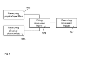
- Fig. 1 shows a diagram of a method for protecting a physical characteristic, e.g. thermal conductivity, of vacuum insulation panels of a certain type.
- the certain type is determined by the structure of the vacuum insulation panels.
- vacuum insulation panels having e.g. a fiber core belong to the same certain type.
- vacuum insulation panels without any core belong to another certain type.
- the method comprises measuring 101 a plurality of physical quantities associated with the vacuum insulation panels at distinct time instants, measuring 103 the radius of the physical characteristic at the distinct time instants, fitting 105 a parametric regression model with the measure of physical quantities as regression parameters in order to predict the measured values of the physical characteristic at the distinct time instants using the parametric regression model.
- the parametric regression model is fitted such that its result yields at least estimates of the measured values of the physical characteristic.
- the method further comprises executing 107, e.g. on a digital computer, the parametric regression model in order to predict the physical characteristic at a future time instant.
- the physical characteristic may be a thermal conductivity, an internal gas pressure or weight.
- the physical quantities may be a temperature or a measured geometry of a vacuum insulation panel etc. The physical quantities are used as regression parameters in order to fit the parametric regression model.
- the physical characteristic of more than 18 vacuum insulation panels may be measured. Thereafter, three groups with respectively 6 VIPs are stored at temperatures of 23°C, 45°C and 70°C. After different time instants, e.g. after 0, 25, 50, 75 or 100 days or after a minimum of 0, 50 or 100 days, the physical characteristic of the VIP may be measured again.
- the measured values may be evaluated using a computer program which is adapted to compute parameter of the parametric regression model using the measuring values in order to provide a prediction of the physical characteristic for e.g. two or ten years at a certain operation temperature.
- the parametric regression model may be a non-linear mixed regression model for predicting efficiency, e.g. thermal conductivity of the VIPs within shorter test intervals, e.g. within 100 days. Nevertheless, the parametric regression model may provide a prediction of a physical characteristic after 15 years within a confidence interval. Thus, the vacuum insulation panels may be tested within 100 days or less in order to obtain a prediction for the physical characteristic or for the change of the physical characteristic over a significantly longer period of time.
- the statistical approach yields more reliable predictions and enables an efficient deployment of test VIPs. Moreover, less VIPs may be used for measurements so that the measurement complexity is reduced.
- vacuum insulation panels having a fiber core are subject to stronger requirements relating to the quality of vacuum than vacuum insulation panels having a silicic acid core.
- VIPs with a fiber core are evacuated during manufacturing by a factor of 100 more than VIPs with other cores.
- the outer skins of the VIPs shall be correspondingly tighter.
- the prediction of the physical characteristic of vacuum insulation panels may be performed in order to estimate how many VIPs have after two years a thermal conductivity which is less then 0.008 W/(mK), or how many VIPs have after ten years a thermal conductivity which is less then 0.015 W/(mK).
- the confidence interval may be set to 95% and 99% at standard environmental conditions, e.g. 24°C and 50% air moisture or 15° Celsius and 50% relative air moisture.
- the maximum temperature may be set to 75° Celsius, the minimal temperature may be set to -40°C, the maximum air moisture may be 98% of the relative air moisture at 5°C.
- a start value for the thermal conductivity forming an embodiment of a physical characteristic may be 0.006 W/(mK).
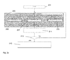
- Fig. 2a shows a diagram of a method for predicting a physical characteristic of more than 18 VIPs.
- the physical characteristic e.g. an inner pressure, weight or thermal conductivity
- groups with more than 6 VIPs are stored at different temperatures, e.g. at a first temperature at 23°C in step 205, a second temperature at 45 to 55°C in step 207 and at a third temperature at 60 to 80°C in step 209.
- the physical characteristics such as the inner pressure, weight or thermal conductivity, is measured again.
- the elapsed time is determined.
- step 215 the measurements are evaluated in order to perform the fitting of a parametric regression model enabling the prediction of the physical characteristic of the vacuum insulation panels at a future time instant, e.g. after 15 years.
- the operational temperature may be set to 20°C.
- the fitting the parametric regression model and the executing the same may be performed using a graphical user interface as shown in Fig. 2b .
- the graphical user interface may implement the regression model 217 which calculates and outputs model parameters.
- the graphical user interface may further comprise a section 219 for predicting a physical characteristic of a vacuum insulation panel, e.g. after two and after ten years.
- the physical characteristic may be the inner pressure or thermal conductivity.
- the graphical user interface may further visualize predicted values versus observed values, 221, observed values versus residuals, 223, predicted values versus residuals, 225, and residuals versus frequency, 227.
- the panel lifetime is defined as the time until panel failure.
- the panel fails if the value of the thermal conductivity exceeds a prescribed critical bound c ⁇ .
- the occurrence of an exceedance over a critical bound c ⁇ is identified with the death of the panel.
- Relevant critical bounds for thermal conductivity are between 0.008 W/(m ⁇ K) after 2 years and 0.015 W/(m ⁇ K) after 10 years.
- thermal conductivity is essentially a function of panel internal gas pressure and internal water content (mass).
- panel failure can be alternatively defined as the exceedance of the panel interior gas pressure and/or the panel internal water content over prescribed critical values.
- thermal conductivity ⁇ gas (t) at time t and gas pressure p gas (t) at time t can be expressed by the following equations.
- ⁇ gas p gas ⁇ free gas 1 + p 1 / 2 p gas ⁇ ⁇ free gas p 1 / 2 ⁇ p gas
- p gas ⁇ gas ⁇ gas ⁇ p 1 / 2 ⁇ free gas - ⁇ gas ⁇ p 1 / 2 ⁇ free gas ⁇ ⁇ gas
- ⁇ ⁇ p gas t ⁇ gas t ⁇ p 1 / 2 ⁇ free gas - ⁇ gas t - ⁇ gas t 0 ⁇ p 1 / 2 ⁇ free gas - ⁇ gas t 0 ⁇ p 1 / 2 ⁇ free gas ⁇ ⁇ gas t 0 ⁇ p 1 / 2 ⁇ free gas ⁇ ⁇ ⁇ gas t .
- the empirical data base consists in two data sets from experiments.
- the experimental or testing objects were specially prepared small panels with sizes of about 10 cm ⁇ 10 cm ⁇ 1 cm and 20 cm ⁇ 20 cm ⁇ 1 cm, denominated as "test panels".
- test panels two panel brands were used that differed in the types of laminates.
- the panel types, respectively the laminates, are denoted as H and W.
- Panel internal gas pressure and panel mass were measured as experimental responses.
- the experimental factors were geometry, i.e. length of sealing, surface area, and kernel volume, temperature, humidity, and time.
- the panels were stored under various experimental conditions in six different environments resulting from the cross combinations of levels of the factors temperature and humidity. Temperature levels were 25°C, 45°C, or 65°C.
- Humidity levels were either uncontrolled or 75% relative.
- the geometric levels were panels with sizes of about 10 cm x 10 cm x 1 cm and 20 cm x 20 cm x 1 cm. As the number of experimental objects two panel units of each size were observed under each of the 6 experimental conditions defined by the cross combinations of levels of the factors temperature and humidity.
- the measurements of internal gas pressure and mass were taken weekly in the beginning and about every second week later, over about one year.
- the testing panels of type H were successively measured at 17 different times
- the testing panels of type W were successively measured at 10 different times.
- the following combinations of levels of the experimental factors temperature and humidity express stress conditions, which are significantly different from ordinary usage conditions, namely the temperature levels "45°C", "65°C” in cross combination with the humidity level "75% relative". Under the stress conditions described before experimental acceleration is achieved and the experimental responses gas pressure and mass increase more rapidly in time than under normal usage conditions.
- the statistical analysis can be based on a model of the evolution of gas pressure or mass as a function of time, in order to predict the long-term evolution from observations over the short-term experimental period. This is a case for statistical regression analysis.
- Y is the observed response, e.g. panel internal gas pressure or panel mass.
- the vector x contains the levels of explicit influential factors, also called regressors, e.g. geometry, temperature, humidity, time.
- ⁇ is a vector of parameters which can be fitted empirically to a specific phenomenon.
- the fixed function g ( x , ⁇ ) aggregates the effects of the factor levels x and of the parameters ⁇ .
- E [ Y ] g ( x , ⁇ ), and g ( x , ⁇ ) is called mean value function.
- Two regression modeling approaches can be used, namely a multivariate linear model and a nonlinear model.
- Two regression modeling approaches can be used, namely a multivariate linear model and a nonlinear model.
- the confidence interval for ⁇ l is: ⁇ ⁇ l - z ⁇ ⁇ ⁇ ⁇ ⁇ c ll ; ⁇ ⁇ l + z ⁇ ⁇ ⁇ ⁇ ⁇ c ll .
- the parameter estimation in the linear model is provided by many software programs by statistical commercially available packages.
- the model (5) can be applied to artificial regressors x i which are aggregations of the explicit variables geometry, temperature, humidity, time.
- the response variables are:
- x 6 and x 7 describe the permeation of dry gases through the sealing.
- the temperature dependency is assumed to be linear.
- x 8 , x 9 and x 10 describe the permeation of dry gases through the laminate.
- the dependency is assumed to be of second order in temperature.
- x 1 , ., x 5 correspondingly describe the permeation of water vapor which is assumed to be proportional to the external water vapor pressure.
- Both models get along without an intercept.
- the unknown coefficients a 1 , ., a 5 and b 0 , .,b 10 are estimated by means of multi-linear regression using the totality of the given data.
- the goodness of fit is examined. If the goodness of fit is satisfying, predictions about the future behavior of the response variables Y 1 and Y 2 can be made using the estimated model.
- the nonlinear approach is a second regression modeling approaches.
- the estimator ⁇ is approximately normally distributed with the k'-dimensional normal distribution N k ⁇ ⁇ , ⁇ ⁇ 2 ⁇ C ⁇ . If ⁇ ⁇ k ' is a prescribed vector, then ⁇ T ⁇ is approximately distributed as the univariate normal distribution N a ⁇ ⁇ ⁇ , ⁇ ⁇ 2 ⁇ a ⁇ ⁇ C ⁇ ⁇ a .
- the following interval results: ⁇ ⁇ l - z ⁇ ⁇ ⁇ ⁇ ⁇ c ll ⁇ ; ⁇ ⁇ l + z ⁇ ⁇ ⁇ ⁇ ⁇ c ll ⁇ .
- C( ⁇ ) is replaced by C( ⁇ ) and c u ( ⁇ ) by c u ( ⁇ ).
- the estimation uses numerical algorithms, in particular minimization algorithms like the Gauß-Newton or Levenberg-Marquard procedures.
- minimization algorithms like the Gauß-Newton or Levenberg-Marquard procedures.
- the solution requires advanced statistical or mathematical software like Statistica, Minitab, or Mathematica.
- a nonlinear model for increase of gas pressure with dependency on mass is discussed, which is based on an iterative data modeling process.
- a simplifying assumption can be used for the analysis of small test panels with kernels made of fumed silica:
- the model (10) can be simplified with in predictive power by omitting the mass term.
- the latter condition corresponds to the conditions in practice for freezers and refrigerators.
- Table 2 shows parameter estimates for the model (13) including confidence intervals for the estimates for both laminate types.
- the quantities displayed in table 2 are explained as follows:
- the R-squared-value is a measure for the goodness of fit of a model. Possible values lie between 0 and 1. The more the R-squared-value approaches 1 the better is the fit of the model. Both the model for H and the model for W show reasonable R-squared-values. R- and R-squared-values. H W R 0.97982448 0.98932815 R-squared 0.96005601 0.97877019
- Fig. 3 shows observed versus predicted values of pressure increase measured in mbar and how precisely the prediction values of the model match with the observed values. Ideally the points lie on a straight line through the origin with a 100%-slope.
- Fig. 4 shows residuals versus predicted values of pressure increase measured in mbar and Fig. 5 shows residuals versus observed values of pressure increase measured in mbar.
- Fig. 6 shows histograms of the residuals measured in mbar for both laminate H and laminate W.
- the histograms are symmetric around zero and exhibit a shape close to a normal distribution, while statistical inferences based on normal distribution are acceptable.
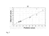
- the model for the increase of pressure which found by fitting the data based on small test panels (about 10 cm ⁇ 10 cm ⁇ 1 cm and 20 cm ⁇ 20 cm ⁇ 1 cm) with laminate H, is tested on the larger panels (about 48 cm ⁇ 48 cm ⁇ 2 cm).
- Fig. 7 shows the predicted values plotted against the observed values of the larger panels. Overestimating the observed values is consistent with the fact that the laminates of the small panels slightly differ from the laminate of the larger panels.
- the response "pressure increase" Y g ( x , ⁇ ) + ⁇ is predicted under usage conditions, i.e. under the following values of the factors, i.e. of the components of x: geometry of usage panels, usually larger than test panels; ambient temperature under usage conditions; and extended time.
- the prediction is based on two components, namely point prediction and interval prediction.
- the interval prediction accounts for the effect of the residual ⁇ .
- Fig. 8 shows the coefficient o( ⁇ ) of the prediction interval (16) as a function of time (measured in years) for panel types H and W.
- testing panels For selection of measuring points the panels are denominated as "testing panels". Each testing panel is measured at three different time points t 1 ⁇ t 2 ⁇ t 3 , i.e. the regressor variable X 5 in model (13) takes three different values.
- Fig. 9 shows the increase in precision of the prediction of pressure increase ⁇ p ⁇ as a function of the duration (measured in days) of the experiment.
- the vertical axis represents the difference in absolute values of two predictions measured in mbar. One is based on all available observations, whereas the other is based on a shorter measuring period with only three measurements. In general the the precision raises the longer the testing panels are kept in the experiment.
- the prediction is for 10 years and 20 °C and panels of size 100 cm ⁇ 50 cm ⁇ 2 cm. To achieve an accuracy of about 2 mbar in the predicted pressure increase of 10 years and 20 °C, panel size 100 cm ⁇ 50 cm ⁇ 2 cm, a minimum measuring time of about 100 days is used.
- Fig. 9 further shows the difference in absolute values between the predicted pressure increase ⁇ p ⁇ measured in mbar based on an estimation of ⁇ from all available observations, measured over the total period of 250 days and respectively 170 days, and predicted values based on an estimation of ⁇ over a shorter period and with only three measurements in time.
- the x-axis depicts the length of this period varied (measured in days). The prediction is for 10 years and 20°C, panels of size 100 cm ⁇ 50 cm ⁇ 2 cm.
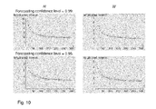
- Fig. 10 shows the relation between the number k of testing panels and the length of the prediction interval (16) for each laminate type in a prediction for temperature 20 °C and 10 years and panels of size 100 cm ⁇ 50 cm ⁇ 2 cm, measured at the beginning and about 50 and 110 days after the first measuring at forecasting confidence levels of 99% and 95%.
- the calculations are based on the parameter estimates ⁇ and variance estimate ⁇ ⁇ ⁇ 2 from the nonlinear regression using all available observations.
- the lengths of the prediction intervals are plotted that result when the estimated variance ⁇ ⁇ ⁇ 2 and its lower ⁇ ⁇ ⁇ L 2 and upper confidence limit ⁇ ⁇ ⁇ U 2 at the 95%-level are used for the calculation, i.e.
- the number of testing panels is set to 60, i.e. the number of experimental units is 10.
- the prediction is for 10 years and 20°C and panels of size 100 cm ⁇ 50 cm ⁇ 2 cm.
- the fit of the nonlinear model (13) with only three parameters is satisfactory and implausible effects are not observed.
- the nonlinear model can be used for extrapolating to lower temperatures. From this point of view the nonlinear model can be used for predictions of the development of pressure along the time axis.
- the univariate model is used below in the context of model validation as a basis of the linearity test by Fisher.
- the data Y i,1 ,..., Y i,m i are observed under a fixed lexel x i of the regressor variable x.
- the data of the larger panels (about 48 cm ⁇ 48 cm ⁇ 2 cm) is analyzed using the model (25).
- the analysis is the univariate special case of the aforementioned method for the multivariate linear model.
- Table 3 shows the estimates of the parameters ⁇ 0 and ⁇ 1 and the residual variance ⁇ ⁇ 2 or the model (25) including confidence intervals at a reliability level of 95%.
- R- and R-squared-values are as follows: Table 3: Empirical results for larger panels. Estimate Lower confidence limit Upper confidence limit ⁇ 0 -6.33 -6.45 -6.22 ⁇ 1 -3780 -4148 -3412 ⁇ 3 31428.7 34488.4 28369 ⁇ ⁇ 2 0.0618179 0.0386411 0.11453 R- and R-squared-values. R 0.96312004 R-squared 0.92760021
- ambient temperature is considered to be room temperature at about 20°C.Humidity is considered to be an uncontrolled experimental factor. Water vapor partial pressure is kept at typical values at ambient temperature. At 20°C, water vapor pressure is about 15 mbar.
- the controlled experimental factors are temperature, geometry, and time elapsed.
- the levels of the controlled factors are as follows:
- the upper temperature level should be tolerably high. At excessively high temperatures phase transitions with additional destructive effects can occur. Concluding from the experience from various measuring experiments, 70°C is appropriate. Water vapor pressure should not exceed values resulting automatically from ambient conditions.
- the increase of pressure can be predicted more precisely the longer the panels are kept in the experiment.
- the length of the prediction interval for the increase of pressure under certain conditions can be considered, to decide how many testing panels should be included in the experiment. Naturally, the length of the prediction interval decreases if the number k of testing panels increses. There might be only a minor decrease in the length of the prediction interval observed for the number k of testing panels ⁇ 120.
- Model (13) assumes the pressure to increase linearly in time when all of the other conditions, namely geometry and temperature, are kept constant.
- Fig. 12 shows an increase in pressure measured in mbar plotted against the elapsed time in days. Each plot shows the three measurements of one testing panel kept under constant conditions depcting a nonlinear relation between pressure increase and elapsed time.
- the three measurements of each testing panel should are visually checked for nonlinearities.
- measuring points can be identified that are not consistent with the assumption of linearity. In this case the panel can be excluded from the experiment and not considered in further examinations.
- Fig. 12 shows two situations for assesing linearity.
- the first plot reveals a higher slope of pressure increase in the beginning than between the second and third measuring.
- the second plot shows a comparibly high third measuring point, which can be an example for the destruction of a testing panel during the experiment due to unsatisfying handling of the panel.
- the pressure increase Y of two panels is measured at three different time points x , namely at the beginning of the experiment, after 57 and after 105 days.
- the following table contains the data: i x i y ij 1 0 0 1 0 0 2 57 2.6 2 57 2.4 3 105 3.3 3 105 3
- the interval prediction accounts for the effect of the residual ⁇ which is not visible in the point estimation.
- the unknown vector ⁇ is replaced by the estimator ⁇ obtained from the actual experiment.
- the estimator is determined by the above described method.
- the bound c ⁇ for the thermal conductivity can be converted into a critical value c for the pressure increase using the following equation, as compared to equations (1) - (3).
- c c ⁇ ⁇ p 1 / 2 ⁇ free gas - c ⁇ - ⁇ gas t 0 ⁇ p 1 / 2 ⁇ free gas - ⁇ gas t 0 ⁇ p 1 / 2 ⁇ free gas ⁇ c ⁇ - ⁇ gas t 0 .
- An initial value ⁇ gas (t 0 ) of the thermal conductivity is either given by the manufacturer of the panels or can be measured at the beginning of the experiment.
- the estimation of parameters in the nonlinear model can be performed with a statistical package.
- the prediction of the proportion nonconforming requires a programming environment.
- Different to kernels made of fumed silica a significant increase in the thermal conductivity with increasing gas pressure not only occurs in the pressure range above 10 mbar, but already in the range of a few tenths of a mbar (see figure 1 ).
- Fig. 13 shows the thermal conductivity for different core materials that are optimized for the application in VIP depending on (nitrogen) gas pressure.
- ⁇ gas p gas ⁇ free gas 1 + / p 1 / 2 p gas ⁇ free gas and p 1/2 are constant properties of the gas and the porous matrix.
- the additional coupling effect especially is pronounced at higher gas pressures, as shown in Fig. 13 by the values between 100 and 1000 mbar.
- the two additional constants a and b can be determined experimentally.
- Fig. 14 the measured thermal conductivity depending on the gas pressure is depicted (circles) for a presumably similar kernel made of glass fibres.
- the X-axis in Fig. 14 is a linear scale, with the pressure range delimitated from 0 to 10 mbar.
- Fig. 2 additionally comprises an analytical description according to the Knudsen formula - dashed line - as well as an empirical description including coupling effects - long dashed line.
- the difference of the two formula descriptions related to the thermal conductivity according Knudsen i.e. a 'relative deviation' - solid line, is related to the right Y-axis.
- Fig. 14 further shows the thermal conductivity of a kernel made of glass fibres depending on the gas pressure: measured values - circles, analytical description according Knudsen formula - dashed line and an empirical description including coupling phenomena - long dashed line.
- the permeating water vapor can be assumed to be adsorbed by dryers or getters on a sufficiently low pressure level so that there is no significant effect on the thermal conductivity.
- the increase of the thermal conductivity is related to penetrating (dry) gases.
- the sensitivity on the gas pressure depends on a characteristic parameter of the filler material p 1/2 , the pressure, at which gas contribution is the half of thermal conductivity of free, non-convecting gas. This parameter is affected by the mean effective pore size.
- Fig. 15 shows a time curve of a measured heat conductivity coefficient.
- the empirical data base consisted in two data sets from experiments. In a first experiment, the measurings showed very small increases in the thermal conductivity in the panel. The experiment had the following characteristics:
- the panels that had initially been stored under 70°C were transferred to a 20°C environment after their second measurement.
- an analysis of panel lifetimes in particular, building a statistical model to enable forecasts of panel lifetime may be performed.
- the panel lifetime is defined as the time until panel failure.
- the panel fails if the value of the thermal conductivity exceeds a prescribed critical bound e c.
- the occurrence of an exceedance over a critical bound is identified with the death of the panel.
- Relevant critical bounds for thermal conductivity are between 0.008 W/(m ⁇ K) after 2 years and 0.015 W/(m ⁇ K) after 10 years.
- the thermal conductivity was measured directly as described.
- the thermal conductivity is essentially a function of panel internal gas pressure.
- thermal conductivity ⁇ gas ( t ) at time t and gas pressure p gas ( t ) at time t are expressed by the following equation.
- ⁇ gas p gas ⁇ free gas 1 + p 1 / 2 p gas ;
- ⁇ free gas 26 x 10-3W/(m ⁇ K) and p 1/2 gas pressure where the (unknown) thermal conductivity equals one half of ⁇ free gas millibar.
- the statistical analysis is based on a model of the heat transfer coefficient, in order to predict the long-term thermal conductivity from observations over the short-term experimental period. This is a case for statistical regression analysis.
- the statistical analysis of experiments on VIPs has to account for two levels of variation:
- each panel is subject to measurement in two periods, see table 5.
- transformed accelerated temperature applied to panel i x temp 20 i x temp , 20 , i x T 20 , i , t - 1 T .
- groups may be defined by panels. If groups are identified with panels, the sampling model uses the following indices and counting variables:
- the location shift can also be allocated to the parameter ⁇ -1'.
- the parameters in the models (7.1), (7.3), (7.4), (7.6), (7.7) and (7.9) can be derived from the tables 3 and 4.
- ⁇ i has the parameters E ⁇ i
- Stochastic variables corresponding to different measuring periods are considered to be independent.
- the family of residual vectors ⁇ z , i ⁇ ⁇ 12,...25 ⁇ ⁇ 23 ⁇ or i ⁇ ⁇ 43. ....51 ⁇ ⁇ ⁇ 47 ⁇ and the family of measurement set-up variation vectors b 1 i ⁇ ⁇ 12, ... 25 ⁇ 23 ⁇ or i ⁇ ⁇ 43 Vietnamese51 ⁇ 47 ⁇ are independent families.
- Cov b i ⁇ b ⁇ 1 2 0 0 ⁇ b ⁇ 2 2 .
- the zeroes of the function h r , a,t are the zeroes of the quadratic function ts 2 y 2 +(2 rst -1) y + r 2 t
- Estimators ⁇ 1 and b 1 i are obtained by equating the coefficient of x in (7.14) with ⁇ 1 i in the fitted linear model (7.26).
- the estimators are obtained by applying the previous results.
- the regression functions of the mixed models as defined can be transformed to conditionally linear model functions.
- Stochastic variables corresponding to different measuring periods are considered to be independent.
- the family of measurement set-up variation vectors b i , i ⁇ ⁇ 12,..., 25 ⁇ ⁇ ⁇ 23 ⁇ or i ⁇ ⁇ 43, ...,51 ⁇ ⁇ ⁇ 47 ⁇ are independent families.
- Table 6 shows the estimates b ⁇ -1 i by equation (7.46) and ⁇ 1 i by equation (7.40), arranged or measurement periods associated to the same panel number, see table 7. Strong ariation comes from the panels, the measurement periods have minor influence only.
- the estimators previously developed depend on prescribed values of he arameters ⁇ 0 and ⁇ 2 .
- Fig. 16 shows that the estimator ⁇ -1 is particularly sensitive to the choice of ⁇ 2.
- N - 2 ⁇ M ⁇ S ⁇ 2 has the ⁇ 2 distribution ⁇ 2 ( N - 2 M ) with degree of freedom N - 2 M .
- X i is a n i ⁇ q i design matrix of known regressor values.
- the q-dimensional random parameter ⁇ i follows the equation.
- the random parameter vector b i and the residual vector ⁇ i are independent among each other.
- equation (7.56) describes an ordinary linear model, where Cov ⁇ ⁇ i
- b i ⁇ 2 ⁇ X i ⁇ ⁇ X i - 1 .
- ⁇ ⁇ i ⁇ i - 1 ⁇ ⁇ ⁇ i - d i , see equation (7.64), has the q-variate normal distribution N ⁇ ⁇ , ⁇ 2 ⁇ ⁇ i - 1 ⁇ X i ⁇ ⁇ X i - 1 ⁇ ⁇ i - 1 ⁇ + B .
- Equation (7.71) shows that the sample residual ⁇ i is independent of b i .
- ⁇ i and S Z i 2 are independent, and the pooled variance estimator S Z 2 defined by equation (7.74) is independent of ⁇ 1 ,..., ⁇ m .
- W 1 ,..., W m have anm-variate joint normal distribution.
- the prediction error ⁇ ( x )- Z ( x ) ( ⁇ ( ⁇ - ⁇ - b )) T x and the estimator ⁇ Z ⁇ x - Z x 2 of the prediction error variance are approximately independent.
- the prediction error has a univariate normal distribution with mean 0 and variance ⁇ Z ⁇ x - Z x 2 given by equation (7.97).
- ( ⁇ ( x )- Z ( x ))/ ⁇ ⁇ ( x )- Z ( x ) has the standard normal distribution N(0; 1).
- the previous results can be applied to the analysis of the transformed model equations considered above.
- ⁇ i ⁇ M b i , - 1 2 ⁇ 2 ⁇ i ⁇ M ⁇ i , - 1 , 1 - ⁇ ⁇ i , - 1 , 1 - - ⁇ i , - 1 , 2 ⁇ exp ⁇ i , - 1 , 3 ⁇ ⁇ 2 + 1 M ⁇ l ⁇ M ⁇ l , - 1 , 2 ⁇ exp ⁇ l , - 1 , 3 ⁇ ⁇ 2 2 .
- a first expansion in ⁇ 2 with a co, 20, l not considered as a function of ⁇ 2 will be described.
- the result (7.138) can also be obtained in the following manner.
- the OLS estimator is provided by equation (7.138).
- the approximate validity of the model (7.140) follows from E [b ⁇ i,-1 ( ⁇ 2 )] We consider the model in the conditional situation given ⁇ i , i ⁇ M .
- confidence intervals for ⁇ 2 can be calculated in the way familiar from linear regression analysis.
- a least favourable forecast estimator ⁇ 0 can be defined in the following sense: Choose ⁇ 0 which maximises the forecast ⁇ ( x ) defined by equation (7.145).
- Basis for the evaluation is the data set containing the values of the measurements.
- the parameter ⁇ 0 is searched for in the interval [1; 4]. Furthermore the two location parameters ⁇ 0 and ⁇ -1 are connected in a negative way: The greater the parameter ⁇ 0 (location parameter with reference to the activation energy), the lower the estimated value for ⁇ -1 (location parameter with reference to the gas pressure). Since a negative value for the parameter ⁇ -1 is considered implausible, the parameter ⁇ 0 is regarded plausible only as long as ⁇ -1 is positive.
- Table 5 shows the parameter estimates for the nonlinear mixed model as above described based on the data set containing the values of the measurements. For the estimation, commercially available tools may be used.
- the parameter estimates based on the measurements are compared with the parameter estimates based on the measurements taken from further measurements.
- the objective is to predict the response "thermal conductivity", a d,1 Y with a d,1 the thickness of panel i, under usage conditions, i. e., for special values of the following two influential factors: 1) Time. This factor is contained in the vector x. 2) Temperature. This factor is contained in the matrix ⁇ .
- the prediction is based on two components:
- the prediction variance is basically formed by
- ⁇ ⁇ 2 0.0000143776
- ⁇ ⁇ Z ⁇ x - Z x 2 0.0169387
- x ⁇ ⁇ ⁇ ⁇ m + 1 m ⁇ B ⁇ ⁇ ⁇ ⁇ ⁇ x 0.0168818
- the analysis is based on the mixed model as described.
- the objective is to ensure a prediction of future values which is as exact as possible without neglecting certain external restrictions.
- the empirical basis for the design study is the data set containing the values of the measurements.
- the precision in the prediction is reflected in the length of the prediction interval (7.156).
- the crucial component of the prediction interval is the variance of the prediction, see formula (7.98).
- the objective of an ideal construction of an experimental design is therefore minimising the length of the prediction interval, see formula (7.112).
- the experimental design aims at minimising one of the following functions of the prediction variance keeping in mind the above remarks.
- the prediction is calculated for panels stored for 2 years in a 20°C-environment at a confidence level of 95%:
- the mixed model analysis estimates some parameters for each panel separately, in particular the residual variance (measurement variance). At least three measuring points are necessary to secure the possibility of estimating the measuring variance for each panel. To exceed the unreliable minimum, it is advised to measure each panel at least four times in the course of the measuring period. Since the measuring variance is regarded rather small in general, four measuring points are assumed to be enough. It is advised that the measuring points are arranged in equal distances making use of the whole available measurement period.
- the accuracy of the prediction can be improved most by increasing the number of testing panels.
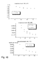
- Fig. 18 shows the length L U - L L of the prediction interval for the transformed values, the contribution ⁇ of the measurement setup to the prediction variance of the transformed values and the length of the prediction interval for the thermal conductivity (unit: W/(mK)) as a function of the number of testing panels. The calculation is based on the following measurement setup:
- the length of the prediction interval is calculated for the following divisions of the panels into the two temperature groups:
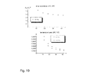
- Fig. 19 shows that a huge improvement in prediction accuracy can be achieved by increasing the number of testing panels involved in the experiment up to a number of about 24. Only a minor improvement can be observed when including more than about 24 testing panels in the experiment.
- Fig. 20 shows the squared length ( L U - L L ) 2 of the prediction interval and the term ⁇ , see equation (8.4), with the intention of comparing the two quantities. It is obvious that ⁇ , which contains the influences of the experimental design, is comparably small in comparison to ( L U - L L ) 2 .
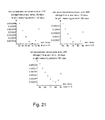
- Fig. 21 shows the component ⁇ of the prediction variance as a function of the length of the overall experimental time. The calculation is based on the following measurement setup:
- Varying the length of the overall experimental time means the following times of measuring:
- Figure 19 shows that strong improvement in ⁇ can be achieved when choosing at least 150 days for the total length of the measuring period.
- the length of the prediction interval in units W/(mK) decreases only little if the measuring period is extended beyond 150 days.
- Figure 20 shows the component ⁇ , see equation (8.3), of the prediction variance as a function of the accelerated temperature level in °C for the three following cases:
- the first plot in Fig. 20 which represents the results for a storage time in the 70°C-environment of 60 days reveals a minimum in ⁇ at an accelerated temperature of about 70°C.
- the second plot representing the results for a storage time in the 70°C-environment of 40 days reveals a minimum in ⁇ at an accelerated temperature of about 80°C. Both plots are based on a measuring period of 120 days.
- the third plot shows the results for a storage time in the 70°C-environment of 40 days with a measuring period of only 100 days. The minimum in ⁇ can be observed at an accelerated temperature of 80°C as well.
- Fig. 20 shows the component ⁇ , see equation (8.3), of the prediction variance as a function of the time the panels are stored in the accelerated environment in days. The calculation is based on the following measurement setup:
- Fig. 20 shows a minimum in ⁇ at a storing time in the 70°C-environment of about 55 days. Hence under the above measurement setup. Fig. 20 suggests that optimally panels should be stored in a 70°C-environment for almost two months before being measured 4 times under room temperature.
- Fig. 21 shows ⁇ as a function of the accelerated temperature level.
- Fig . 22 shows ⁇ as a function of the storage time of the panels in the accelerated environment in days.
- the choice of the experimental design depends on the amount of the variation due to differences in the panel quality. Therefore first of all examinations should be taken on how much the panel-to-panel variation influences the accuracy in the prediction in comparison to the other factors determining the experimental design.
- the accuracy in the prediction can be improved by extending the measuring period.
- a measuring period of at least 150 days should bring reasonable results in the prediction.
- the measurements on panels which are stored under approximately room temperature should begin with the start of the experiment. Panels which are stored in an accelerated environment should first remain in that environment for a prescribed time, and should afterwards being measured. If the panel-to-panel variation is comparably high, a shortening of the measuring period might be justifiable if in return the number of panels is increased.
- each panel may be measured 4 times.
- the measuring points should be equally distributed over the entire measuring period. I. e., for panels stored at room temperature, the first measuring point is the starting time of the experiment, and for panels stored under in an accelerated environment, the first measuring point is the time point right after the end of the accelerated storing period. For both groups of panels, the last measuring point is at the end of the experimental period.
- two temperature levels should be chosen in which the panels are stored during the experiment. Partly the panels are recommended to be stored in an environment of about 25°C which is approximately room temperature. The remaining panels should be stored in an environment of about 70°C if the storing time in the accelerated environment is chosen to be 60 days. If this period is shortened, the acceleration effect can nevertheless be achieved by increasing the accelerated temperature.
- testing panels a number of at least 24 testing panels are recommended to be included in the experiment.
- the panels can be divided into to equally sized groups: one group being stored in a 25°C-environment, and the other in a 70°C-environment. Whether to increase the number of testing panels or rather to increase the length of the measuring period depends on what is the decisive factor for the prediction variance: panel-to-panel variation or the measurement-to-measurement variation.
- the unknown parameter ⁇ 0 has to be replaced by the estimator ⁇ 0 from the actual experiment.
- the estimator is determined as described above.
- the approach to predict the proportion of nonconforming items where the confidence level is not prescribed but random may be deployed.
- the preceding analysis is based on two-sided prediction intervals for the thermal conductivity.
- a prescribed forecasting confidence level ⁇ can be achieved. If the upper bound a d,i Y ⁇ U ( x ) is below the critical value c for the thermal conductivity it can be concluded that in the long run not more than (1 - ⁇ ) ⁇ 100% of the panels are expected to exceed c. Otherwise no conclusion is possible, i. e. the percentage of the panels exceeding the critical values cannot be estimated below 100%.
- This approach allows to decide what percentage of the panels exceed the critical value at the utmost while ensuring a higher confidence level for the prediction than in the case of a two-sided prediction interval. Nevertheless, to ensure the possibility of drawing a conclusion, this method is only recommended if the predicted response is far below the critical value c.
- the basis for the investigations were measurements taken on highly degrading panels with high panel-to-panel variation that are not suitable and cannot be used for the intended purpose. Since the critical values for the thermal conductivity are not far from the point prediction, no conclusion would be possible in many cases if one-sided prediction intervals were used. Therefore, the investigations concentrated on two-sided prediction intervals which allow to estimate an interval with upper and lower bound in which the future observations lie with a high probability. Also, the two-sided interval allows to compare the accuracy of the prediction by means of the length of the prediction interval, and is suitable especially for the construction of an experimental design.
- the initial data basis were measurings. By this means increases in the thermal conductivity could be expected to be measured accurately. At the same time, further measurings were taken for control purposes. In the course of the project, while deriving an optimal experimental design, it was realised that it would be necessary to include a high number of testing panels in future experiments to make precise predictions for the thermal conductivity.
Landscapes
- Physics & Mathematics (AREA)
- Health & Medical Sciences (AREA)
- Life Sciences & Earth Sciences (AREA)
- Chemical & Material Sciences (AREA)
- Analytical Chemistry (AREA)
- Biochemistry (AREA)
- General Health & Medical Sciences (AREA)
- General Physics & Mathematics (AREA)
- Immunology (AREA)
- Pathology (AREA)
- Management, Administration, Business Operations System, And Electronic Commerce (AREA)
Abstract
Description
- The invention relates to predicting a physical characteristic of vacuum insulation panels in the future upon the basis of measurements.
- Vacuum insulation panels are widely used for thermal insulation of home appliances and buildings. However, the physical characteristics such as thermal conductivity of vacuum insulation panels tend to change over time. In order to capture the changing physical characteristics, long time measurements may be performed. However, in view of a long lifetime of typical vacuum insulation panels - 10 years and more - it is not feasible to perform measurements over that long period of time.
- It is therefore the object of the present invention to provide an efficient concept for determining a physical characteristic such as thermal conductivity of vacuum insulation panels for a long period of time.
- This object is achieved by the features of the independent claim. Further embodiments are disclosed in the figures, in the description and in the dependent claims.
- The invention is based on the finding that the above object may be solved by predicting future physical characteristic of vacuum insulation panels upon the basis of a parametric regression model.
- According to an aspect, the invention relates to a method for predicting a physical characteristic of vacuum insulation panels of a certain type, the method comprising measuring a plurality of physical quantities associated with the vacuum insulation panels at distinct time instants, measuring values of the physical characteristic at the distinct time instants, fitting a parametric regression model with the measured physical quantities as regression parameters to predict the measured values of the physical characteristic at the distinct time instants using the parametric regression model, and executing the parametric regression model to predict the physical characteristic at a future time instant. The future time instant is a time instant following the certain time instants.
- According to an embodiment, the parametric regression model is executed and/or fitted by a computer.
- According to an embodiment, the parametric regression model is a non-linear regression model, in particular a mixed non-linear regression model.
- According to an embodiment, the values of the physical characteristic and the plurality of physical quantities are measured at three distinct time instants, in particular only at three distinct time instants.
- According to an embodiment, the physical characteristic is a least one of: thermal conductivity, internal gas pressure, weight.
- According to an embodiment, the measured physical quantities are at least one of the following physical quantities: temperature, elapsed time during which a vacuum insulation panel was exposed to a certain test condition, in particular to a certain temperature, geometry of a vacuum insulation panel, in particular a sealing length or a surface area or a volume of a kernel of a vacuum insulation panel or a thickness of a vacuum insulation panel, a mass of a vacuum insulation panel, a relative mass increase of a vacuum insulation panel.
- According to an embodiment, the step of fitting of the parametric regression model comprises determining regression coefficients of the parametric regression model.
- According to an embodiment, the method further comprises determining the distinct time instants for measurements.
- According to an embodiment, the method further comprises determining a number of vacuum insulation panels of the same type for measurements.
- According to an embodiment, the method further comprises determining a total measurement time of the measurements.
- According to an embodiment, the method further comprises determining environmental conditions, in particular temperatures, to which to expose at least one vacuum insulation panel.
- According to an embodiment, the method further comprises determining an exposure time.
- According to an embodiment, the method further comprises determining a number of measurements repetitions.
- According to an embodiment, the vacuum insulation panel of the same type comprises a panel core, in particular a fiber panel core.
- According to an embodiment, the parametric regression model is one of the following parametric regression models

or
with Y denoting values of the physical characteristic, β1 - β4 denoting regression coefficients, x1 - x4 denoting measured values of the physical characteristic and ε denoting an error. - According to an embodiment, the parametric regression model is described by a nonlinear function.
- According to an embodiment, the predicting the physical characteristic of the vacuum insulation panels comprises predicting a number of vacuum insulation panels having a certain value of the physical characteristic or having a value of the physical characteristic below or above a threshold.
- According to an embodiment, the predicting the physical characteristic of the vacuum insulation panels comprises predicting a change of the physical characteristic over time. Further embodiments of the invention will be described with respect to the following figures, in which:
- Fig. 1
- shows a diagram of a method for protecting a physical characteristic;
- Fig. 2a
- shows a diagram of a method for predicting a physical characteristic of more than 18 VIPs;
- Fig. 2b
- shows a graphical user interface;
- Fig. 3
- shows observed versus predicted values of pressure increase;
- Fig. 4
- shows residuals versus predicted values of pressure increase;
- Fig. 5
- shows residuals versus observed values of pressure increase;.
- Fig. 6
- shows histograms of the residuals;
- Fig. 7
- shows predicted values plotted against observed values of larger panels.
- Fig. 8
- shows a coefficient of a prediction interval;
- Fig. 9
- shows an increase in precision of a prediction of pressure increase;
- Fig. 10
- shows a relation between the number of testing panels and a length of the prediction interval;
- Fig. 11
- shows a sensitivity of the coefficient of the prediction interval;
- Fig. 12
- shows an increase in pressure measured in mbar plotted against the elapsed time in days;
- Fig. 13
- shows the thermal conductivity for different core materials;
- Fig. 14
- shows the thermal conductivity of a kernel made of glass fibres.
- Fig. 15
- shows a measured heat conductivity;
- Fig. 16
- shows a characteristic of an estimator;
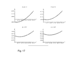
- Fig. 17
- shows estimates;
- Fig. 18
- shows estimates;
- Fig. 19
- shows a prediction variance;
- Fig. 20
- shows a prediction variance;
- Fig. 21
- shows a prediction variance; and
- Fig. 22
- shows a prediction variance.
-
Fig. 1 shows a diagram of a method for protecting a physical characteristic, e.g. thermal conductivity, of vacuum insulation panels of a certain type. The certain type is determined by the structure of the vacuum insulation panels. Thus, vacuum insulation panels having e.g. a fiber core belong to the same certain type. Correspondingly, vacuum insulation panels without any core belong to another certain type. - The method comprises measuring 101 a plurality of physical quantities associated with the vacuum insulation panels at distinct time instants, measuring 103 the radius of the physical characteristic at the distinct time instants, fitting 105 a parametric regression model with the measure of physical quantities as regression parameters in order to predict the measured values of the physical characteristic at the distinct time instants using the parametric regression model. In other words, the parametric regression model is fitted such that its result yields at least estimates of the measured values of the physical characteristic.
- The method further comprises executing 107, e.g. on a digital computer, the parametric regression model in order to predict the physical characteristic at a future time instant.
- The physical characteristic may be a thermal conductivity, an internal gas pressure or weight. Correspondingly, the physical quantities may be a temperature or a measured geometry of a vacuum insulation panel etc. The physical quantities are used as regression parameters in order to fit the parametric regression model.
- According to an embodiment, the physical characteristic of more than 18 vacuum insulation panels (VIP) may be measured. Thereafter, three groups with respectively 6 VIPs are stored at temperatures of 23°C, 45°C and 70°C. After different time instants, e.g. after 0, 25, 50, 75 or 100 days or after a minimum of 0, 50 or 100 days, the physical characteristic of the VIP may be measured again. The measured values may be evaluated using a computer program which is adapted to compute parameter of the parametric regression model using the measuring values in order to provide a prediction of the physical characteristic for e.g. two or ten years at a certain operation temperature.
- The parametric regression model may be a non-linear mixed regression model for predicting efficiency, e.g. thermal conductivity of the VIPs within shorter test intervals, e.g. within 100 days. Nevertheless, the parametric regression model may provide a prediction of a physical characteristic after 15 years within a confidence interval. Thus, the vacuum insulation panels may be tested within 100 days or less in order to obtain a prediction for the physical characteristic or for the change of the physical characteristic over a significantly longer period of time.
- The statistical approach yields more reliable predictions and enables an efficient deployment of test VIPs. Moreover, less VIPs may be used for measurements so that the measurement complexity is reduced.
- When predicting the physical characteristic of vacuum insulation panels, the type of vacuum insulation panels is an important factor. By way of example, vacuum insulation panels having a fiber core are subject to stronger requirements relating to the quality of vacuum than vacuum insulation panels having a silicic acid core. In particular, VIPs with a fiber core are evacuated during manufacturing by a factor of 100 more than VIPs with other cores. Thus, the outer skins of the VIPs shall be correspondingly tighter.
- In order to support a low gas pressure, additional integrated dry means may be used in the vacuum insulation panels. It has been found that VIPs with fiber core suffer from non-linear effects influencing a degradation of the physical characteristics, such as thermal conductivity of the VIP.
- According to an embodiment, the prediction of the physical characteristic of vacuum insulation panels may be performed in order to estimate how many VIPs have after two years a thermal conductivity which is less then 0.008 W/(mK), or how many VIPs have after ten years a thermal conductivity which is less then 0.015 W/(mK). The confidence interval may be set to 95% and 99% at standard environmental conditions, e.g. 24°C and 50% air moisture or 15° Celsius and 50% relative air moisture. The maximum temperature may be set to 75° Celsius, the minimal temperature may be set to -40°C, the maximum air moisture may be 98% of the relative air moisture at 5°C. A start value for the thermal conductivity forming an embodiment of a physical characteristic may be 0.006 W/(mK).
-
Fig. 2a shows a diagram of a method for predicting a physical characteristic of more than 18 VIPs. Instep 201, the physical characteristic, e.g. an inner pressure, weight or thermal conductivity, is measured. Thereafter, instep 203, groups with more than 6 VIPs are stored at different temperatures, e.g. at a first temperature at 23°C instep 205, a second temperature at 45 to 55°C instep 207 and at a third temperature at 60 to 80°C instep 209. Thereafter, instep 211, after 25, 50, 75 or 100 days, at least with three measurement time instants by 0, 50 and 100 days, the physical characteristics, such as the inner pressure, weight or thermal conductivity, is measured again. Instep 213, the elapsed time is determined. If the elapsed time is greater than 100 days, then the method proceeds withstep 215. Instep 215, the measurements are evaluated in order to perform the fitting of a parametric regression model enabling the prediction of the physical characteristic of the vacuum insulation panels at a future time instant, e.g. after 15 years. Instep 215, the operational temperature may be set to 20°C. - According to an embodiment, the fitting the parametric regression model and the executing the same may be performed using a graphical user interface as shown in
Fig. 2b . The graphical user interface may implement theregression model 217 which calculates and outputs model parameters. The graphical user interface may further comprise asection 219 for predicting a physical characteristic of a vacuum insulation panel, e.g. after two and after ten years. The physical characteristic may be the inner pressure or thermal conductivity. The graphical user interface may further visualize predicted values versus observed values, 221, observed values versus residuals, 223, predicted values versus residuals, 225, and residuals versus frequency, 227. - The following describes a statistical model for predicting panel lifetime. The panel lifetime is defined as the time until panel failure. The panel fails if the value of the thermal conductivity exceeds a prescribed critical bound c̃. The occurrence of an exceedance over a critical bound c̃ is identified with the death of the panel. Relevant critical bounds for thermal conductivity are between 0.008 W/(m·K) after 2 years and 0.015 W/(m·K) after 10 years.
- However, thermal conductivity is essentially a function of panel internal gas pressure and internal water content (mass). Hence panel failure can be alternatively defined as the exceedance of the panel interior gas pressure and/or the panel internal water content over prescribed critical values.
- The functional relationships between thermal conductivity λ gas(t) at time t and gas pressure pgas(t) at time t can be expressed by the following equations.


- The constants are λ free gas = 25.5 × 10⁻³ W/(m·K) and p 1/2 = 650+/-100 mbar. The conversion of the critical bound c̃ for thermal conductivity into a critical bound c for gas pressure can be calculated using equation (27).
- The empirical data base consists in two data sets from experiments. The experimental or testing objects were specially prepared small panels with sizes of about 10 cm × 10 cm × 1 cm and 20 cm × 20 cm × 1 cm, denominated as "test panels". Regarding the quality of experimental objects two panel brands were used that differed in the types of laminates. The panel types, respectively the laminates, are denoted as H and W. Panel internal gas pressure and panel mass were measured as experimental responses. The experimental factors were geometry, i.e. length of sealing, surface area, and kernel volume, temperature, humidity, and time. The panels were stored under various experimental conditions in six different environments resulting from the cross combinations of levels of the factors temperature and humidity. Temperature levels were 25°C, 45°C, or 65°C. Humidity levels were either uncontrolled or 75% relative. The geometric levels were panels with sizes of about 10 cm x 10 cm x 1 cm and 20 cm x 20 cm x 1 cm. As the number of experimental objects two panel units of each size were observed under each of the 6 experimental conditions defined by the cross combinations of levels of the factors temperature and humidity.
- Regarding experimental period and distribution of measuring times the measurements of internal gas pressure and mass were taken weekly in the beginning and about every second week later, over about one year. In view of the number of measurements per experimental object the testing panels of type H were successively measured at 17 different times, whereas the testing panels of type W were successively measured at 10 different times. The following combinations of levels of the experimental factors temperature and humidity express stress conditions, which are significantly different from ordinary usage conditions, namely the temperature levels "45°C", "65°C" in cross combination with the humidity level "75% relative". Under the stress conditions described before experimental acceleration is achieved and the experimental responses gas pressure and mass increase more rapidly in time than under normal usage conditions. This acceleration effect was exploited for building a model for long-term prediction of the evolution of gas pressure and mass from observations from a period of one year only. For model validation purposes, a second data set of measurements on larger panels (about 48 cm x 48 cm x 2 cm) was considered.
- In spite of the stress conditions, the responses gas pressure and mass never reached critical bounds corresponding to critical thermal conductivity levels between 0.008 W/(m·K) and 0.015 W/(m·K).
- Several statistical methods and approaches are explored for modeling panel lifetime.
- An analysis of the probability distribution of lifetime is a customary approach in statistical lifetime modeling. The statistical theory of lifetime and reliability has developed a great variety of parametric classes of lifetime distribution. Most popular is the class of Weibull- distributions. In recent years, the empirical analysis of lifetime distributions from accelerated experiments under stress conditions has made considerable progress.
- The empirical modeling of a lifetime distribution requires the empirical observation of lifetimes, such as times until death, i.e. times until exceedance of critical bounds. In the underlying experiment the responses of the gas pressure and mass never reached critical bounds corresponding to critical thermal conductivity levels between 0.008 W/(m · K) and 0.015 W/(m · K).
- If panel failure (panel death) is not able to be observed, the statistical analysis can be based on a model of the evolution of gas pressure or mass as a function of time, in order to predict the long-term evolution from observations over the short-term experimental period. This is a case for statistical regression analysis. The general form of a parametric regression model is

- Y is the observed response, e.g. panel internal gas pressure or panel mass. The vector x contains the levels of explicit influential factors, also called regressors, e.g. geometry, temperature, humidity, time. β is a vector of parameters which can be fitted empirically to a specific phenomenon. The fixed function g(x, β) aggregates the effects of the factor levels x and of the parameters β. The residual ε expresses random deviation due to non-explicit factors like measurement uncertainty or manufacturing variation in the panels. The residual is supposed to have no effect on the average, i.e. E[ε] = 0 is assumed. Hence E[Y] = g(x, β), and g(x, β) is called mean value function. Two regression modeling approaches can be used, namely a multivariate linear model and a nonlinear model. Two regression modeling approaches can be used, namely a multivariate linear model and a nonlinear model.
- The multivariate linear regression model as a first model is an instance of the general scheme (4) where

I.e. the mean value function is a linear function g(x, β) = β1 x 1 + ... + β kxk . - The following parameters are estimated:
- 1) the components of the vector β, where the estimator is denoted as β̂; and
- 2) the
variance 

- For a specific data set the random effects model is Yi = βT xi + ε i , i = 1,..., n, and in vector notation:
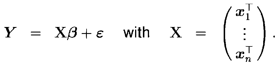
β = (β1,.., β k')T is the vector of the regression parameters. - The k' × k'-matrix C is defined by

the existence of the inverse provided. - The least squares estimator β̂ is determined from the
equations 
- The confidence interval for β l is:

- The
variance 

- The parameter estimation in the linear model is provided by many software programs by statistical commercially available packages.
- The model based prediction for the value Y (x) = βT x + ε x is Ŷ (x) = β̂T x. The prediction interval for the true value Y (x) = βT x + ε x is

with

- The model (5) can be applied to artificial regressors xi which are aggregations of the explicit variables geometry, temperature, humidity, time.
- The underlying explicit untransformed regressor variables are:
- geometrical regressor variables: length of seal, e.g. for the special test panels 2(lF + bF ) with lF and bF the lengths of the seal at the long the panel, surface area of the panel, e.g. for the special test panels it was 2 · lF · bF , volume of the kernel, e.g. for the special test panels it was lK · bK · hK with lK and bK and hK the lengths of the different sides of the kernel;
- ambient regressor variables: temperature ϑ (in °C), relative humidity F (in %);
- measuring time t in days; and
- current mass m(t), current pressure p(t).
- The response variables are:
- relative mass increase Y 1 = (m(t) - m(t 0))/m(t 0), where t0 is the starting time of measuring, m(t) is mass at time t in grams, and m(t0 ) is the initial mass at to; and
- absolute pressure increase Y2 = p(t) - p(t 0), where p(t) is the pressure at time t in mbar, and p(t0 ) is the initial pressure at t 0.
- The following aggregated regressor variables are calculated:
- Explanatory variables of first order:
- F 1 = lK · b K ·hK (volume kernel)
- F 2 = 2 · (lF + bF ) (length of sealing)
- F 3 = 2 · (lF ·bF + bF · hF + lF · hF ) (surface area of the panel)1
- F 4 = 6.1078 · exp(17.08 · ϑ/(234.18 + ϑ)) · F/100 (partial pressure of water vapour in the environment)
- F 5 = m(t 0) (initial mass)
- F 6 = t - t 0 (elapsed measuring time)
- F 7 = ϑ (temperature)
- Explanatory variables of second order:
- x 1 = F 2 · F 4 · F 6/F 5
- x 2 = F 2 · F 4 · F 6/F 5 · F 7
- x 3 = F 3 · F 4 · F 6/F 5
- x 4 = F 3 · F 4 · F 6/F 5 · F 7
-

- x 6 = F 2 · F 6/F 1
- x 7 = F 2 · F 6/F 1 · F 7
- x 8 = F 3 · F 6/F 1
- x 9 = F 3 · F 6/F 1 · F 7

- x 6 and x 7 describe the permeation of dry gases through the sealing. The temperature dependency is assumed to be linear. x 8, x 9 and x 10 describe the permeation of dry gases through the laminate. The dependency is assumed to be of second order in temperature. x 1, .,x5 correspondingly describe the permeation of water vapor which is assumed to be proportional to the external water vapor pressure.
- By means of the above explanatory variables the response variables can be approximately described by the following two linear models:
- Model of the relative increase in mass (Y1):

- Model of the increase in pressure (Y2) (by dry air and water vapor):

- Both models get along without an intercept. The unknown coefficients a 1, .,a 5 and b0, .,b10 are estimated by means of multi-linear regression using the totality of the given data. The goodness of fit is examined. If the goodness of fit is satisfying, predictions about the future behavior of the response variables Y1 and Y2 can be made using the estimated model.
- The fit of the linear model with explanatory variables up to second order is good in the region of experimental factor levels, i.e. geometry, temperature, humidity.
- The nonlinear approach is a second regression modeling approaches.
- This modeling approach is based on a regression model Y = g(x,β) + ε of type (4) with nonlinear mean value functions g(x,β). Firstly the theory of the statistical analysis of such nonlinear regression models is reviewed, which is applied below.
- The following parameters are estimated:
- 1) the components of the vector β, where the estimator is denoted as β̂ ; and
- 2) the
variance 

- For a specific data set the random effects model is Yi = g(xi ,β) + ε i , i = 1,..., n, and in vector notation

with
- β = (β1,..., β k')T is the vector of the regression parameters and X = (x 1,..., xn )T the matrix of the regressor values.
- The n × k' -matrix G(X,β) is defined by

- The k ' × k' -matrix C(β) is defined by

the existence of the inverse provided. - The least squares estimator β̂ is determined from the
equations 
- For a large sample size n the estimator β̂ is approximately normally distributed with the k'-dimensional normal distribution
 k' is a prescribed vector, then αTβ̂ is approximately distributed as the univariate normal distribution


with

- For the empirical analysis C(β) is replaced by C(β̂).
- The confidence interval for β l is obtained by predefining the vector α l = (0,..., 0, 1, 0,...., 0)T, with α l = 1 as its /-th component and the components α j = 0 for j ≠ l. The following interval results:

- For the empirical analysis C(β) is replaced by C(β̂) and c u (β) by c u (β̂).
- The
variance 

- The estimation uses numerical algorithms, in particular minimization algorithms like the Gauß-Newton or Levenberg-Marquard procedures. The solution requires advanced statistical or mathematical software like Statistica, Minitab, or Mathematica.
- The model based prediction for the value Y(x) = g(x,β) + ε x is Ŷ(x) = g(x.β̂). If


with

- For the empirical analysis C(β) is replaced by C(β̂) and d(β) by d(β̂).
- The confidence intervals and prediction intervals given by formulae (7) and (8) are based on linear approximations of the mean value function g(x, β), compared to equation (4). In the following the mean value function is strictly monotonous in all parameters.
Table 1: Notation of variables and coefficients in the nonlinear regression model. variable meaning model notation model coefficient LS length of the sealing - - A = AFolie surface area - - V volume of the kernel - - 
length of sealing per volume x 1 cLS - β1 
surface per volume x2 cA - β2 
transformed temperature x3 E = β3 t - t0 time elapsed x 5 - 
relative mass increase x 4 α = β4 - In the following the aforementioned methods are applied to the prediction of pressure and mass increase.
- A nonlinear model for increase of gas pressure with dependency on mass is discussed, which is based on an iterative data modeling process. A simplifying assumption can be used for the analysis of small test panels with kernels made of fumed silica:
- 1. Permeation through edges and corners is assumed to be negligible, so that the coefficients c air,C , c air,LE , cwv,C and c wv,LE are assumed to be zero.
- 2. The driving force for permeation of air is the external pressure. The variation of internal pressure is neglected.
- 3. The internal water vapor partial pressure is assumed to be constantly zero, consequently there are no effects due to saturation.
- 4. The variation of temperature is assumed to follow an Arrhenius equation.
- 5. The effect of temperature on the permeation is the same for length of the sealing and surface area.
- The assumptions result in the model

with R = 8.314472 (J/(mol K)) being the gas constant, T the temperature in K, E the activation energy, cLS the coefficient of the sealing, cA the coefficient of the surface area and α the coefficient of the mass. The reference temperature is T0 = 296.15 K. The values E, cLS , cA , α are unknowns. - Equation (9) expresses the relation between the increase in pressure and the above mentioned parameters on average. When the model empirically is fitted, the random deviation can be considered. If Y is the observed increase in gas pressure, then equation (9) corresponds to the regression model

with
- See above for a survey of the used notation. The residual ε in equation (10) expresses the random deviation due to nonsystematic measuring effects and due to manufacturing and handling effects of the panels.
- Therefore the fit of the model is performed by means of nonlinear regression analysis.
- Here the gradient


- A nonlinear model for increase of gas pressure without dependency on mass is discussed.
- Under consideration of the panels under low water vapor partial pressure the model (10) can be simplified with in predictive power by omitting the mass term. The latter condition corresponds to the conditions in practice for freezers and refrigerators. The following regression model is considered:

with
- See above for a survey of the used notation used. The fit of the model is performed by means of nonlinear regression analysis. If the gradient
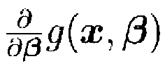

Table 2: Empirical results for small test panels. Parameter estimates for panels with laminate H. Estimate Lower confidence limit Upper confidence limit β1 cLS 0.001174 0.000941 0.001407 β2 cA 0.0186 0.0157 0.0215 

3677 3487 3866 β3 E 30572.3 28992.6 32143.7 
0.356300 0.295745 0.437672 Parameter estimates for panels with laminate W. Estimate Lower confidence limit Upper confidence limit β1 c LS 0.001067 0.000845 0.001290 β2 c A 0.0216 0.0186 0.0245 

3282 3107 3458 β3 E 27288.1 25833.1 28751.4 
0.0870747 0.0684527 0.114527 - In an empirical fit of the nonlinear model without mass term the following parameters are estimated:
- 1) the components of the vector β, as explained by formula (14). The estimator is denoted as β̂; and
- 2) the
variance 

- For the estimation, commercially available tools in combination with the minimization algorithm of Levenberg-Marquard can be used.
- Table 2 shows parameter estimates for the model (13) including confidence intervals for the estimates for both laminate types. The quantities displayed in table 2 are explained as follows:
- Estimate is an empirical estimate of the parameter from the measurement data.
- Lower/Upper confidence limit represents two values L < U such that with a high probability, here 0.95, the true value of the estimated parameter lies between L and U.
- The R-squared-value is a measure for the goodness of fit of a model. Possible values lie between 0 and 1. The more the R-squared-value approaches 1 the better is the fit of the model. Both the model for H and the model for W show reasonable R-squared-values.
R- and R-squared-values. H W R 0.97982448 0.98932815 R-squared 0.96005601 0.97877019 -
Fig. 3 shows observed versus predicted values of pressure increase measured in mbar and how precisely the prediction values of the model match with the observed values. Ideally the points lie on a straight line through the origin with a 100%-slope. -
Fig. 4 shows residuals versus predicted values of pressure increase measured in mbar andFig. 5 shows residuals versus observed values of pressure increase measured in mbar. -
Fig. 4 andFig. 5 plot the residual ε = observed values predicted values of H and W against the predicted values and the observed values, respectively. For W-type and H-type panels the plots show agreement and predictive power of the model. -
Fig. 6 shows histograms of the residuals measured in mbar for both laminate H and laminate W. The histograms are symmetric around zero and exhibit a shape close to a normal distribution, while statistical inferences based on normal distribution are acceptable. - The model for the increase of pressure, which found by fitting the data based on small test panels (about 10 cm × 10 cm × 1 cm and 20 cm × 20 cm × 1 cm) with laminate H, is tested on the larger panels (about 48 cm × 48 cm × 2 cm).
-
Fig. 7 shows the predicted values plotted against the observed values of the larger panels. Overestimating the observed values is consistent with the fact that the laminates of the small panels slightly differ from the laminate of the larger panels. - For a model based prediction the nonlinear model (13) integrates three types of influential factors expressed by the vector x:
- 1) geometry (sealing length, surface area, volume);
- 2) temperature; and
- 3) time.
- Experiments are performed under specific factor levels, like small test panels, accelerated temperature, relatively short time. Under these conditions, the model aforementioned parameters are estimated.
- The response "pressure increase" Y = g(x,β) + ε is predicted under usage conditions, i.e. under the following values of the factors, i.e. of the components of x: geometry of usage panels, usually larger than test panels; ambient temperature under usage conditions; and extended time.
- The prediction is based on two components, namely point prediction and interval prediction.
- The point prediction is a prediction of the expected value Ŷ = g(x, β̂), ignoring random deviation effects expressed by the residual ε.
- The interval prediction accounts for the effect of the residual ε. The structure of the interval prediction is


-
Fig. 8 shows the coefficient o(β̂) of the prediction interval (16) as a function of time (measured in years) for panel types H and W. The prediction is for a temperature of 20 °C andpanel size 100 cm × 50 cm × 2 cm. Since multiplying this coefficient by the variance σ̂ε of the residual ε and

- Experimental design under the nonlinear approach is discussed under consideration of the nonlinear model (13).
- For selection of measuring points the panels are denominated as "testing panels". Each testing panel is measured at three different time points t1 < t2 < t3, i.e. the regressor variable X5 in model (13) takes three different values.
- In this case it is possible to reveal occasional problems and disturbances in the measuring process. A reasonable distribution of measuring points is to measure at the beginning of the experiment and after two equally sized time intervals. Accordingly t1 is the starting time of the experiment and t2 = 0.5 (t1 + t3). The time length of the experiment is determined by the comparison of the following calculations:
- 1) The increase of pressure in a panel is predicted by the value g(x,β̂) of the nonlinear regression function (13), where x is the prediction point with respect to the regression factors and where β is estimated from all available observations.
- 2) The increase of pressure in a panel is predicted by the value of the nonlinear regression function (13), where x is the prediction point with respect to the regression factors, and where β is estimated from the observations at three selected time points more or less equidistant in time. Additionally the time period is varied.
-
Fig. 9 shows the increase in precision of the prediction of pressure increase Δp̂ as a function of the duration (measured in days) of the experiment. The vertical axis represents the difference in absolute values of two predictions measured in mbar. One is based on all available observations, whereas the other is based on a shorter measuring period with only three measurements. In general the the precision raises the longer the testing panels are kept in the experiment. The prediction is for 10 years and 20 °C and panels ofsize 100 cm × 50 cm × 2 cm. To achieve an accuracy of about 2 mbar in the predicted pressure increase of 10 years and 20 °C,panel size 100 cm × 50 cm × 2 cm, a minimum measuring time of about 100 days is used. -
Fig. 9 further shows the difference in absolute values between the predicted pressure increase Δp̂ measured in mbar based on an estimation of β̂ from all available observations, measured over the total period of 250 days and respectively 170 days, and predicted values based on an estimation of β̂ over a shorter period and with only three measurements in time. The x-axis depicts the length of this period varied (measured in days). The prediction is for 10 years and 20°C, panels ofsize 100 cm × 50 cm × 2 cm. - The choice and number of testing panels and the statistical sample size is calculated from the following components:
- The number of independently varying factors is three, namely temperature, geometry, time. The humidity remains uncontrolled at ambient levels. The numbers of levels of these factors are: 3 levels of temperature, 2 geometric levels, 3 time levels, as compared to above.
- Each of the 3 × 2 = 6 combinations of temperature and geometry requires 1 testing panel. Observations at the 3 time levels are taken for each panel. Hence each experimental unit should use 3x2 = 6 panels.
- In order to guarantee the validity of the experiment in case of unexpected events like improper or destroyed material, the minimum number of experimental units should be 2, i.e. 2x6 = 12 panels.
- The number of experimental units can be successively increased starting from 2. If q is the total number of experimental units, then q = 2, 3, 4
- The number of panels for q experimental units is qx6. Each new experimental unit can use 6 additional testing panels.
- The total statistical sample size n counts all measurements. Under q experimental units, each of the qx6 panels is measured at 3 time points. Hence the statistical sample size is n = qx6x3 = q×18. Each new experimental unit uses 6x3 = 18 additional measurements.
- Under a statistical sample size n, the required number of testing panels is k=n/3. In order to decide how many testing panels should be included in the experiment, the length of the prediction interval for the increase of pressure under certain conditions can be considered.
-
Fig. 10 shows the relation between the number k of testing panels and the length of the prediction interval (16) for each laminate type in a prediction fortemperature 20 °C and 10 years and panels ofsize 100 cm×50 cm×2 cm, measured at the beginning and about 50 and 110 days after the first measuring at forecasting confidence levels of 99% and 95%. The calculations are based on the parameter estimates β̂ and variance estimate


-
Fig. 11 shows the sensitivity of the coefficient o(β̂) of the prediction interval (16) to the estimation of the parameters β1 = cLS (coefficient of the sealing), β2 = cA (coefficient of the surface area) and
size 100 cm × 50 cm × 2 cm. Only one parameter β i , i = 1, 2, 3 is varied at the same time in the range of its confidence interval, whereas the other two parameters β j , j = 1, 2, 3, j ≠ i are kept constant. The coefficient of the prediction interval changes is constant when varying the parameter estimates. Therefore the assumption the performed experiment with the small test panels of types H and W is a representative for experiments of that kind, since the coefficient o(β̂) of the prediction interval (16) and thus also the length of the prediction interval, are hardly sensitive to slight changes of the parameter estimates. - The fit of the nonlinear model (13) with only three parameters is satisfactory and implausible effects are not observed. In particular the nonlinear model can be used for extrapolating to lower temperatures. From this point of view the nonlinear model can be used for predictions of the development of pressure along the time axis.
- Linearity testing under a univariate linear regression model without intercept is discussed. The univariate linear regression model without intercept is a special case of model (5) with k = 1, i.e. with only one regressor variable × and only one coefficient β. The model equation for the response Y is

- In the analysis of the panel internal gas pressure Y , the univariate regression model(18) arises as an instance of the nonlinear model (13)


model (13) collapses into the model according to (18). - The univariate model is used below in the context of model validation as a basis of the linearity test by Fisher. The procedure of the Fisher-test is explained in general. Having a phenomenon with random response Y , the hypothesis

of the validity of model (18) is to be tested. The empirical data base consists of N = m1 + ... + mh observations Y assembled in the h groups Yij, i = 1,..., h, j = 1,..., mi. For each group i, the data Yi,1 ,...,Yi,mi are observed under a fixed lexel xi of the regressor variable x. One requirement for Fisher's test of linearity is the assumption, that mi ≥2 for at least one i=1, .,h, i.e. for at least one level x¡ of the regressor variable we have more than one observation. - Fisher's test proceeds in the following steps:
- 1) Determine the customary least squares estimate β̂ for β .This estimate is implemented as "univariate regression analysis without intercept" in every reasonable statistical package and even in EXCEL.
- 2) Determine the interpolations Ŷi = β̂ x
i for i = 1,..., h. - 3) For i = 1, ..., h determined the arithmetical mean

- 4) Calculate the residual sum of
squares 
- 5) Calculate the replication sum of
squares 
- 6) Calculate the lack of fit sum of
squares 
- 7) The hypothesis H: Y = βx + ε of the validity of model (18) can be rejected at a confidence level of γ · 100% if the test
statistic 
is greater than or equals z F(h-1,N-h) (γ), which is the γ-quantile of the F-distribution F(h - 1, N - h) with h-1 and N-h degrees of freedom. γ usually is chosen as γ=0.95 or γ=0.99. If the test statistic (23) does not exceed or equals z F(h-1,N-h) (γ), then the hypothesis H: Y = βx + ε cannot be rejected. - An analysis of originally sized mass production panels is discussed
- For the analysis of originally sized mass production panels geometric effects are irrelevant. Hence the mean value function g(x,β) of the model (13) can be linearized by considering the logarithm of g(x,β) :

- This leads to considering the linear model

with
- The data of the larger panels (about 48 cm × 48 cm × 2 cm) is analyzed using the model (25). The analysis is the univariate special case of the aforementioned method for the multivariate linear model. Table 3 shows the estimates of the parameters θ0 and θ1 and the residual
variance 
- The R- and R-squared-values are as follows:
Table 3: Empirical results for larger panels. Estimate Lower confidence limit Upper confidence limit θ0 -6.33 -6.45 -6.22 θ1 -3780 -4148 -3412 β3 31428.7 34488.4 28369 
0.0618179 0.0386411 0.11453 R- and R-squared-values. R 0.96312004 R-squared 0.92760021 - Operating instructions for small test panels are discussed.
- Regarding choice of the experimental factors and their levels ambient temperature is considered to be room temperature at about 20°C.Humidity is considered to be an uncontrolled experimental factor. Water vapor partial pressure is kept at typical values at ambient temperature. At 20°C, water vapor pressure is about 15 mbar.
- The controlled experimental factors are temperature, geometry, and time elapsed. The levels of the controlled factors are as follows:
- Temperature, two level model: The lower temperature level is close to usage conditions. Hence, for practical reasons tolerable lower levels are close to ambient temperature, e. g. 20°C.
- The upper temperature level should be tolerably high. At excessively high temperatures phase transitions with additional destructive effects can occur. Concluding from the experience from various measuring experiments, 70°C is appropriate. Water vapor pressure should not exceed values resulting automatically from ambient conditions.
- Temperature, three level model: Upper and lower levels are chosen as in the two level model. An intermediate temperature is chosen as the Arrhenius mean of the lower and upper level. For instance, the Arrhenius mean of the
lower level 20°C and theupper level 70 °C is about 55 °C. - Geometry: Two levels are achieved by varying the sealing length. The surface varies implicitly in the sealing length. The levels should be clearly distinct in the sense that the ratios of sealing length versus surface area differ substantially between the two levels. The experimental vacuum chamber restricts the linear extension of the test panels, typically at a maximum of 30 cm. For instance, the above analysed experiments ar perforemd with test panels of
kernel extensions 10 cm × 10 cm (level one) and 20 cm × 20 cm (level two). - Time elapsed: Each panel should me measured at three different time points t1<t2 <t3. A reasonable distribution of measuring points is to measure at the beginning of the experiment and after two equally sized time intervals. For example t1 is the starting time of the experiment, and t2 = 0.5(t1 + t3).
- In general the increase of pressure can be predicted more precisely the longer the panels are kept in the experiment. To achieve an accuracy of about 2 mbar in the predicted pressure increase in a prediction for 10 years and 20° C and
panel size 100 cm × 50 cm × 2 cm, t3≥100 days can be chosen. - The choice of the number of testing panels is discussed.
- In order to cover all combinations of independently varying controlled factors like temperature, geometry and time, when the temperature has 3 and the
geometry 2 levels, at least 3x2 = 6 testing panels (= 1 experimental unit) are used. Each testing panel is measured at 3 time levels. A minimum number of experimental units can be 2, i.e. 2× 6 = 12 panels. The number of experimental units can be increased starting from 2, where each new experimental unit uses 6 additional testing panels and 18 additional measurements. The total number of measurements is summarized in the statistical sample size n and the statistical sample size is n = q×6×3 = q×18. - The length of the prediction interval for the increase of pressure under certain conditions can be considered, to decide how many testing panels should be included in the experiment. Naturally, the length of the prediction interval decreases if the number k of testing panels increses. There might be only a minor decrease in the length of the prediction interval observed for the number k of testing panels ≥ 120.
- A test of linearity is discussed.
- Measurements can be checked for plausibility. Model (13) assumes the pressure to increase linearly in time when all of the other conditions, namely geometry and temperature, are kept constant.
-
Fig. 12 shows an increase in pressure measured in mbar plotted against the elapsed time in days. Each plot shows the three measurements of one testing panel kept under constant conditions depcting a nonlinear relation between pressure increase and elapsed time. - The three measurements of each testing panel should are visually checked for nonlinearities. When plotting the pressure increase against the elapsed time, measuring points can be identified that are not consistent with the assumption of linearity. In this case the panel can be excluded from the experiment and not considered in further examinations.
-
Fig. 12 shows two situations for assesing linearity. The first plot reveals a higher slope of pressure increase in the beginning than between the second and third measuring. The second plot shows a comparibly high third measuring point, which can be an example for the destruction of a testing panel during the experiment due to unsatisfying handling of the panel. - A formal test of linearity is discussed.
- When considering the nonlinear model (13) given by


- Hence a test for the validity of the univariate model H : Y = βx + ε under fixed panel size and fixed temperature can also provide a test for the validity of the nonlinear model (13). At least 2 equally sized panels are observed under a fixed temperature. Hence the requirements for Fisher's formal test of linearity described are satisfied. An application of the test is illustrated by the following example.
- The pressure increase Y of two panels is measured at three different time points x, namely at the beginning of the experiment, after 57 and after 105 days. The following table contains the data:
i xi y ij1 0 0 1 0 0 2 57 2.6 2 57 2.4 3 105 3.3 3 105 3 - The hypothesis is H: Y = βx. There are h = 3 time points and N = 6 observations m i =2 for i = 1, 2, 3, because at each time point there are 2 measurements (1 for each panel). The replication sum of squares is

- Performing a linear regression on the data results in an estimation of β = 0.0331547. In the following table the replication averages y̅ i as well as the predicted values ŷi and the residuals ĉij are given.
i xi yij y̅i ŷi ε̂ij 1 0 0 0 = (0+0)/2 0 0 1 0 0 0 = (0+0)/2 0 0 2 57 2.6 2.5 = (2.6+2.4)/2 1.88982 0.510183 2 57 2.4 2.5=(2.6+2.4)/2 1.88982 0.710183 3 105 3.3 3.15=(3.3+3)/2 3.48124 -0.481242 3 105 3 3.15=(3.3+3)/2 3.48124 -0.181242 - The residual sum of squares is

- Thus the sum of squares due to lack of fit is

- Therefore the test statistic takes the
value 
- Further the value of the 95%-quantile of the F(2,3)-distribution is 5.78614. Since 22.2482 > 5.78614, the hypothesis that there is a linear relation of the form Y = βx between Y and x can be rejected at a condidence level of 0.95.
- Prediction of the proportion of nonconforming items is discussed.
- To predict the proportion of nonconforming items, the point prediction Ŷ(x) for the pressure increase as well as the prediction interval

can be examined. The interval prediction accounts for the effect of the residual ε which is not visible in the point estimation. By suitable choice of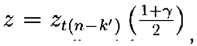


I.e. the probability that the real pressure increase value Y lies in the interval Bx is γ. The prediction interval for the widely used forecasting confidence levels γ =0.95 and γ = 0.99 is considered. - If the upper bound

- If the upper bound of the prediction interval for γ = 0.99 is higher than the critical value c, then the prediction interval for γ = 0.95 can be calculated. If the upper bound of the prediction interval is below c, in the long run less than 5% of the panels exceed the critical value c.
- To predict the proportion of nonconforming items, consider the following two cases:
- 1) Ŷ(x) < c, i.e. the point prediction Ŷ(x) lies below the critical value c. In this case the upper bound


with
- 2) Ŷ(x) > c ,i.e. the point prediction Ŷ(x) lies above the critical value c. In this case the lower bound


with
- The unknown vector β is replaced by the estimator β̂ obtained from the actual experiment. The estimator is determined by the above described method.
- In industrial applications, bounds c̃ for the absolute value of the thermal conductivity are prescribed, e.g. c̃ = 0.008 W/(m·K) after 2 years and c̃ = 0.015 W/(m · K) after 10 years. The bound c̃ for the thermal conductivity can be converted into a critical value c for the pressure increase using the following equation, as compared to equations (1) - (3).

- The constants are λfree gas = 25.5 × 10⁻³ W/(m·K) and p 1/2 = 650+/-100 mbar. An initial value λ gas(t0) of the thermal conductivity is either given by the manufacturer of the panels or can be measured at the beginning of the experiment.
- The estimation of parameters in the nonlinear model can be performed with a statistical package. In particular, the prediction of the proportion nonconforming requires a programming environment.
For the description of the physical basics on heat transfer in vacuum insulation panels, as well as on degradation effects due to penetrating gases see Report ZAE 2 - 1108 - 12 (2008). Different to kernels made of fumed silica a significant increase in the thermal conductivity with increasing gas pressure not only occurs in the pressure range above 10 mbar, but already in the range of a few tenths of a mbar (seefigure 1 ). - Accordingly, for low degradation rates in the insulation capability vacuum tight envelopes with penetration rates of a factor of 10 to 100 smaller can be used.
-
Fig. 13 shows the thermal conductivity for different core materials that are optimized for the application in VIP depending on (nitrogen) gas pressure. - A coupling effect considerably at kernels made of glass fibres is taken into account. In the evacuated state dot-like contacts between single glass fibres yield high thermal resistances. In the non-evacuated state this contact resistance is bypassed by the gas. Consequently a total thermal conductivity results that is larger than expected for the sum of the thermal conductivity of the evacuated specimen and the thermal conductivity of the free, non-convecting gas:

with
λ tot being the total thermal conductivity;
λevac being the thermal conductivity of the evacuated material;
λ gas being the contribution of the gas according Knudsen formula (see below);
and
λ coupl an additional coupling term. - According to considerations done by Knudsen the contribution of the gas to the total thermal conductivity depending on the gas pressure p gas can be described by:

λ free gas and p 1/2 are constant properties of the gas and the porous matrix. - The additional coupling effect especially is pronounced at higher gas pressures, as shown in
Fig. 13 by the values between 100 and 1000 mbar. The contribution of the coupling effect is taken into account in a modified empirical equation:
- The two additional constants a and b can be determined experimentally.
- In
Fig. 14 the measured thermal conductivity depending on the gas pressure is depicted (circles) for a presumably similar kernel made of glass fibres. The X-axis inFig. 14 is a linear scale, with the pressure range delimitated from 0 to 10 mbar.Fig. 2 additionally comprises an analytical description according to the Knudsen formula - dashed line - as well as an empirical description including coupling effects - long dashed line. The difference of the two formula descriptions related to the thermal conductivity according Knudsen, i.e. a 'relative deviation' - solid line, is related to the right Y-axis. -
Fig. 14 further shows the thermal conductivity of a kernel made of glass fibres depending on the gas pressure: measured values - circles, analytical description according Knudsen formula - dashed line and an empirical description including coupling phenomena - long dashed line. The difference between the two formula descriptions related to the thermal conductivity according Knudsen that are referred to as 'relative deviation', is related to the right Y-axis - solid line. - The increase of the internal gas pressure that causes the degradation of the thermal performance of the vacuum insulated panel - VIP - is linearly in time. In contrast to kernels made of fumed silica at accelerated tests of VIP with glass fibre kernels the internal gas pressure increases up to a pressure region, at which the increase of the thermal conductivity can be no longer considered as linearly with gas pressure. Thus the nonlinearity due to 'saturation' according Knudsen formula can be taken into account. Experimental tests as well as analyses can be limited to the pressure range below 10 mbar. Within this region the thermal conductivity increases up to a value of approximately 0.020 W/(m·K), which is a value that cannot be reached in practical application even at longer service time. Within this region the influence of the coupling effect remains below 4%. Thus in the following considerations the coupling effect can be neglected.
- The permeating water vapor can be assumed to be adsorbed by dryers or getters on a sufficiently low pressure level so that there is no significant effect on the thermal conductivity.
- Regarding the used physical regression model the increase of the thermal conductivity is related to penetrating (dry) gases. The sensitivity on the gas pressure depends on a characteristic parameter of the filler material p 1/2, the pressure, at which gas contribution is the half of thermal conductivity of free, non-convecting gas. This parameter is affected by the mean effective pore size.
- Whether a larger increase is caused by a higher permeability of the envelope or whether it is caused by a higher sensitivity of the filler material due to larger effective pores, cannot precisely determined. In the regression model rates of increase of gas pressure and initial gas pressure are given in multiples of p 1/2.
- From the measurements it can also not determined precisely, whether higher or different values of the thermal conductivity measured at the beginning of the tests are related to different thermal conductivity of the evacuated kernels or whether they are related to different internal gas pressures significantly affecting the total thermal conductivity.
-
Fig. 15 shows a time curve of a measured heat conductivity coefficient. - In the following, the empirical basis of the measurements will be described.
- The empirical data base consisted in two data sets from experiments. In a first experiment, the measurings showed very small increases in the thermal conductivity in the panel. The experiment had the following characteristics:
- Experimental objects: The experimental or testing objects were specially prepared small panels of one brand with sizes of about 35 cm x 35 cm x 1 cm
- Measured experimental responses: heat transfer coefficient
- Experimental factors: temperature, time
- Experimental conditions: The panels were stored under two different temperature levels: 20°C (non-accelerated condition), 70°C (accelerated condition)
- Number of experimental objects: 8 test panels
- Experimental setting: 4 test panels under constant 20°C (non-accelerated condition). Four test panels temporarily under 70°C (accelerated condition), temporarily under 20°C (non-accelerated condition).
- Experimental period: 01.10.2008 until 23.04.2009
- Measurement method: 6 among the 8 panels were subject to measurements twice over the experimental period
- Distribution of measuring times: Each measurement of the heat transfer coefficient was extended over a time period between 3 and 31 days. During each period the heat transfer coefficient in a panel is measured every 5 minutes, so that all in all for each measuring period between about 800 and 9000 observations are available
- Stress conditions: The storage temperature of 70°C is considered as a stress condition that is not expected to occur in practice
- Experimental acceleration: The stress conditions described before allow the estimation of the activation energy which can be used for the prediction of the heat transfer coefficient when storing the panels under arbitrary temperatures
- One measuring run (panel 46 = measuring
run number 13, see table 5) of a panel showed results considerably different from all other measuring results. It was concluded that the panel was delivered with defects, for which reason it was not measured a second time and is not considered in further analysis. Furthermore the second panel which was not measured twice is excluded from the analysis (panel 51 = measuring run number 19). So in the sequel only a total of six panels, each with 2 measuring runs, is considered. - In addition, further measurements have been performed. For control purposes, the absolute values of the heat transfer coefficient were measured twice for each test panel during the experimental period. The specifications of this second measurement experiment are as follows:
- Experimental objects: The experimental or testing objects were specially prepared small panels of one brand with sizes of about 35 cm x 35 cm x 1 cm.
- Measured experimental responses: heat transfer coefficient
- Experimental factors: temperature, time.
- Experimental conditions: The panels were stored under two different temperature levels: 20°C (non-accelerated condition), 70°C (accelerated condition).
- Number of experimental objects: 10 test panels
- Experimental setting: 5 test panels under constant 20°C (non-accelerated condition). 5 test panels temporarily under 70°C (accelerated condition), temporarily under 20°C (non-accelerated condition).
- Experimental period: 01.10.2008 until 23.04.2009
- Measurement method: Each of the 10 panels was measured three times during the experimental period. Each measurement took about half a day.
- Distribution of measuring times: Each of the panels was measured in the beginning, after a period of 50 to 70 days and at the end of the experimental period.
- The panels that had initially been stored under 70°C were transferred to a 20°C environment after their second measurement.
- Stress conditions: The storage temperature of 70°C is considered as a stress condition that is not expected to occur in practice.
- Experimental acceleration: The stress conditions described before allow the estimation of the activation energy which can be used for the prediction of the heat transfer coefficient when storing the panels under arbitrary temperatures.
- The panel which in the measurements showed considerably different results from the other panels (panel 46, see table 5) also showed high degradation rates in the measurements. It is excluded from the further analysis based on the measurements.
- According to an embodiment, an analysis of panel lifetimes, in particular, building a statistical model to enable forecasts of panel lifetime may be performed. The panel lifetime is defined as the time until panel failure. The panel fails if the value of the thermal conductivity exceeds a prescribed critical bound e c. The occurrence of an exceedance over a critical bound is identified with the death of the panel. Relevant critical bounds for thermal conductivity are between 0.008 W/(m· K) after 2 years and 0.015 W/(m· K) after 10 years.
- In the present context, the thermal conductivity was measured directly as described. However, the thermal conductivity is essentially a function of panel internal gas pressure.
- The functional relationships between thermal conductivity λgas(t) at time t and gas pressure p gas(t) at time t are expressed by the following equation.

- The constants are λ free gas = 26 x 10-3W/(m· K) and p 1/2 gas pressure where the (unknown) thermal conductivity equals one half of λ free gas millibar.
- The total thermal conductivity λ gesamt = Y = λ gas + β evac due to the influence of the gas pressure therefore results in the regression model

With
β evac = thermal conductivity of the completely evacuated panel; β-1 = initial gas pressure; β0 = p 1/2, β1 = c, β2 = E (activation energy);

t = time in days;
T, = temperature in K;
R = gas constant; R = 8:314472(J/(mol K));
T 0 = reference temperature; T0 = 296:15 K: - There are basically 2 levels of temperatures: 20°C and 70°C. For each panel i, each point of time t let TN,i,t be the exact temperature, the panel j ist stored in temperature level N between t and t + 1.
- For each panel i, each time point t and each temperature level N let d(i; t;N) be the storage period of panel i until t in the temperature level N and

the average temperature in the temperature level N. - In the following, regression models will be described.
- The statistical analysis is based on a model of the heat transfer coefficient, in order to predict the long-term thermal conductivity from observations over the short-term experimental period. This is a case for statistical regression analysis. The statistical analysis of experiments on VIPs has to account for two levels of variation:
- 1) Measurement-to measurement variation in runs of repeated measurements,
- 2) panel-to-panel variation resulting from manufacturing instability.
- Because of the immaturity of the VIP manufacturing sector, panel-to-panel variation is particularly strong and serious. The subsequent study accounts for the above requirements by analysing experiments on VIPs by a nonlinear mixed regression model. Such models are often referred to as hierarchical nonlinear regression models.
- With respect to mixed models, he basic modeling problem is to distinguish between variation resulting from panels and variation resulting from measurement. For a better understanding of this distinction, a sampling model is much more instructive than a structural model.
- As to the distinction of groups, one has to distinguish groups of measurement taken under similar conditions. Two factors are relevant: the panels and the measurement periods. The factor "measurement period" is more distinctive. In general, each panel is subject to measurement in two periods, see table 5.
- Groups defined by measurement periods. If groups are identified with measurement periods, the sampling model uses the following indices and counting variables:
• Group index i of measurement periods, i ∈ M = {12,...,25}\{23}.
• The sample size n i in group i is the number n i of measurements during measurement period i.
• Index j of measurements. In measurement period i, j ranges over j = 1; :::; ni.Table 3: Parameters of the models (7.1), (7.3), (7.4), (7.6), (7.7) and (7.9). β0 thermal conductivity in the evacuated and dry state of the panel β-1 β-1 = p 0.'p: 2 average initial relative gas pressure in a panel art time 0 β1 β, = c, p, 2 average increase of relative gas pressure per day β2 activation energy β vector of 3-regression coefficients b 0i random deviation of the initial thermal conductivity of panel i from the population average b -.i random deviation of the initial relative gas pressure of panel i from the population average biz random deviation of the increase of relative gas pressure of panel i from the population average per day b 2 vector of random deviations of panel i from the population average x time.20 it total non-accelerated exposure timeof panel i until measurement j in days T̅Nit average temperature of panel i at the time point t in temperature group N in K T 0 T 0 = 296.13 K reference temperature atemp 70 i 
x temp 20 i 
aco,20,i 
a time,70 i total accelerated exposure time of panel i adi thickness of the panel i a i a i = (ai , a timp 70.i, a time 70 i ) vector of the levels of the observable factors varying only with the groups i and not with measurement time j Table 4: Parameters of the models (7.1), (7.3), (7.4), (7.6), (7.7) and (7.9). x i, j xi,j = (x temp 20 i.j · x time 20 i,j )- vector of the levels of the observable factors varying with the groups i and with measurement time j in days εi,j measurement errors or measurement residuals ε i εi = (εi,1, ..., εi,n i )- collection of measurement errors εi......εi ni Y i Y i = (Yi,1;.....Yi,n , T vector of the ni measurements obtained in group iR universal gas constant R = 8.314472 J x mol-1 × K-1 λ free gas thermal conductivity λ free gas = 26 · 10-3 W × m-1 × K -1 of the free and still gas - Furthermore, groups may be defined by panels. If groups are identified with panels, the sampling model uses the following indices and counting variables:
- Group index i of panels, i ∈ M = {43..... 51} \ {47}.
- The sample size n i, in group i is the number n 1 of measurements taken on panel i.
- Index j of measurements taken on the panel. With respect to panel i, j ranges over
- In the following, a mixed model with random shift in location will be described.
- The mixed nonlinear regression model with a random location shift b0i for each group i ∈ {12....25}\{23} or i ∈ {43.....51}\{47} is based in the following equations:


- For i ∈ {12,...,25}\ {23} or i ∈ {43,..., 51}\{47}, j = 1,..., ni .
- In the following, a fixed model with random shifts in location and slope will be described.
- The mixed nonlinear regression model with a random location shift b 0i and a random shift b 1i in the slope for each group i ∈ {12,...,25}\{23} or i ∈ {43,..., 51}\{47} is based on the following equations:


- For i ∈{12,...,25}\{23} or i ∈ {43,...,51}\{47}, j = 1,...,n i.
- In the following, a second mixed model with random shifts in location and slope will be described.
- The location shift can also be allocated to the parameter β-1'. The mixed nonlinear regression model with a random location shift b-1i and a random shift b 1i in the slope for each group i ∈ {12,...,25}\{23} or i ∈ {43,..., 51} \ {47} is based in the following equations:


- For i ∈ {12,..., 25}\{23} or i ∈ {43,..., 51}\{47}, j = 1,..., n i.
- In the following, the parameters in the mixed models (7.1), (7.3) and (7.4), (7.6) will be described.
- The parameters in the models (7.1), (7.3), (7.4), (7.6), (7.7) and (7.9) can be derived from the tables 3 and 4.
- Further comments on the parameters:
- Approximately, T̅ 20,i,j = 293.0, hence

Obviously, the variation of xtemp,20,i,j is too small to allow the estimation of the activation energy β2 from panels stored under non-accelerated temperature only. From prior physical knowledge, values 4·104 ≤ β2 ≤ 5·104 are to be expected. The gas constant R is R = 8.314472 (J/(mol K)). Hence
- The random parameters are collected in the vector b i = (b 0i )T for model (7.3), b i = (b 0i,b1i )T, for model (7.6) and bi = (b -1i ,b 1i) T, for model (7.6), respectively. If groups are defined by measurement periods, the vectors bi, i ∈ {12,..., 25} \{23} express variation due to different panels and different measurement set-ups. If groups are defined by panels, the vectors bi, i ∈ {43, ..., 51} \ {47} express variation due to different panels.
- In the following, stochastic assumptions on the mixed models (7.1), (7.3) and (7.4), (7.6) will be described.
- For each measurement period i, the residual vector εi and the vector of measurement set-up deviations are considered to be independent. In particular, ε i has the parameters

- Stochastic variables corresponding to different measuring periods are considered to be independent. In particular, the family of residual vectors εz, i ∈ {12,...25} \{23} or
i ∈ {43. ....51} · {47} and the family of measurement set-up variation vectors
b 1i ∈ {12, ... 25}\{23} or i ∈ {43.....51}\{47}, are independent families. - The measurement set-up variation vectors b2, i ∈ {12.....25}\{23}, are considered to be i.i.d. with parameters

- From equations (7.11) and (7.12) we have

Table. 5: Panels and measurement periods panel number number 1 st measuring period number 2nd measuring period storing 43 16 24 at 20° C 44 17 25 45 18 26 46 13 - 47 - - after first 48 14 20 measuring 49 12 21 storing at 50 15 22 70°C 51 19 - 52 - - - In the following, linear expansion of model equations will be described.
- When all other parameters and variables are kept fixed, the regression function f(xij ; ai; β; bi) of model (7.4) grows nearly linearly in x time 20 i j'. To simplify the investigation, we approximate f(xi ,.u 2.β.b 1) by its linear expansion around x time 20 i j = 0. The derivative is

- In particular

- The approximation by linear expansion around x time,20,i,j = 0 provides

- In the following, an application of the approximation (7.14) for panels stored under non-accelerated conditions will be described.
- For the panels stored under non-accelerated conditions (approximately 20 °C), we have a time,70,i = 0, hence the approximation

- In the following, an application of the approximation (7.14) for panels stored under accelerated conditions will be described.
- For a simple application of the approximation (7.14) for panels stored under accelerated conditions (approximately 70 °C), we need a further approximation. Let τ,s > 0 and consider the function

for y > -τ/s. - Then

- In particular

- Hence we obtain the approximations

for small |y|. |β1 + b 1i | is expected to be small. With
we obtain from (7.16)
- Inserting these approxiomations into (7.14), we obtain the approximation

for i ∈ M 70'. for i ∈ M 20 we have a time,70.i = 0. Hence (7.17) can also be used to express the approximation (7.15) for i ∈ M 20. - In the following, shift estimations based on the approximation (7.17) of the model equation will be described.
- In the subsequent approach, the parameters β-1 and β2 in model (7.4) are considered as prescribed. We fit univariate linear models

to the data from groups i to obtain the OLS estimates α̃ 0i , α̃ 1i . Using the approximations (7.15) and (7.17), we can develop estimators for β0, β1, and for the shift quantitities b 0i , b 1i . Motivated by E[b 0i ] = 0 = E[b 1i ], estimators b̂ 0i , i ∈ M, and b̂ 1i , i ∈ M, are required to satisfy
- In the following, an estimation of β1 and b 1i will be described. (7.15), (7.17), and (7.18) suggest the
estimator 
for β1 + b 1i . Application of the summation rule (7.19) provides the estimator
- For β1. Hence

- Estimates b 1i ,
- In the following, estimation of β0 and b 0i , will be described. (7.15), (7.17), and (7.18) suggest the
estimator 
for β0 + b 0i . Application of the summation rule (7.19) provides the estimator
- For β0. Hence

estimates b 0i . - In the following, shift estimations based on the approximation (7.14) of the model equation will be described.
- In the subsequent approach, the parameters β-1 and β2 are considered as prescribed. We fit univariate linear models

to the data from groups i to obtain the OLS estimates α̂0i, α̂1i . Using the approximation (7.14), we can develop estimators for β0, β1, and for the shift quantitities b 0i , b 1i , Motivated by E[b 0i ] = 0 = E[b 1i ], estimators b̂ 0i , i ∈ M, and |b̂ 1i, i ∈ M, are required to satisfy
- In the following, a basic equation will be discussed.
- We consider the function

- In case of s = 0, the function h r,a,t has the unique zero y r,a,t = r 2 t. In case of s > 0, the zeroes of the function h r,a,t are the zeroes of the quadratic function ts 2 y 2+(2rst-1)y+r 2 t The discriminant of the quadratic equation ts 2 y 2+(2rst-1)y+r 2 t = !0 is


- Where


- Hence the unique zero y r,a,t = r 2 t from the case s = 0 is approximated by


- In the following, estimation of β1 and b1i will be described.
- Estimators β1 and b 1i are obtained by equating the coefficient of x in (7.14) with α̂1i in the fitted linear model (7.26). The resulting equation is

- or
equivalently 
- The estimators are obtained by applying the previous results.
In case of a temp,70,i = 0, we obtain
- In case of

- We obtain

- In the following, a transformation to linear model will be described.
- The regression functions of the mixed models as defined can be transformed to conditionally linear model functions.
- In the following, a transformation of the mixed model (7.4) will be described.
- Consider the regression function f(xij ,ai , β, bi ) of the mixed model (7.4) with random shifts in location and slope. Then

- Conditionally under β0i = β0 + b0i , and for given value of β2, the model


is a linear regression model in x time,20,i,j', where the coefficients α0i, α1i are linear functions of the parameters β-1 and β1i = β1 + b 1i - In the following, a transformation of the second mixed model (7.7) will be described.
- Consider the regression function f(xij ,α i ,β,bi ) of the second mixed model (7.7) with random shifts in location and slope. Then
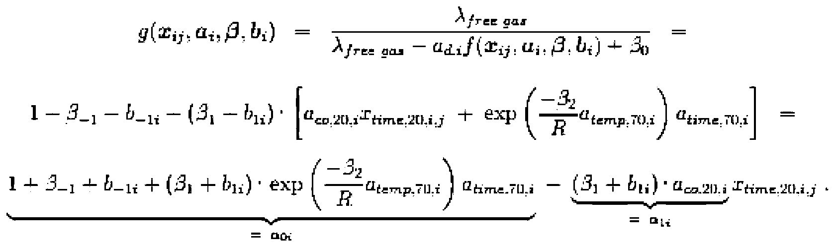
- For given values of β0 and of β2, the model


is a linear regression model in x time,20,i,j , where the coefficients α0i , α1i are linear functions of the parameters β-1 + b -1i and β1i = β1 + b 1i . - In the following, a stochastic assumptions on the mixed model (7.33), (7.34) will be described.
- For each measurement period i, the residual vector ε i and the vector of measurement set-up deviations are considered to be independent. In particular, the vector ε Zi = (ε Zi1,..., ε Zin
i )T has the parameters
- Stochastic variables corresponding to different measuring periods are considered to be independent. In particular, the family of residual vectors ε Zi , i ∈ {12,..., 25} \ {23} or i ∈ {43, ..., 51} \ {47}, and the family of measurement set-up variation vectors bi , i ∈ {12,..., 25} \ {23} or i ∈ {43, ...,51} \ {47}, are independent families.
- The measurement set-up variation vectors b i, i ∈ {12, ..., 25} \ {23}, are considered to be i.i.d. with parameters

- From equations (7.33) and (7.35) we have


- In the following, estimations based on the transformed model equation will be described.
- We consider the transformed mixed models (7.33), (7.34). In the subsequent approach, he parameters β0 nd β2 re considered as prescribed. We fit the linear model described y (7.33), (7.34) to the data from groups i to obtain the OLS estimates α̂0i , α̂1i . Estimators of β-1i and β1i are obtained by equating the respective expressions in formula (7.34) to he estimates α̂0i, α̂1i . Motivated by E[b -1i ] = 0 = E[b 1i ], estimators b̂ -1i , i ∈ M, and b̂ 1i , i ∈ M are required to satisfy

- In the following, an estimation of β1 and b 1i will be described.
- The estimator for β1i is

- Application of the summation rule (7.39) provides the estimator

for β1. The estimators for the b 1i are
- From the structure of the mixed model (7.33), (7.34), and from the theory of univariate egression, we have E[α̂1i |b1i ](β1 + b1i )α∞,20,i , hence E[α̂1i ] = β1α∞,20,i, hence

- Hence ! b̂ 1i is a linear unbiased predictor of b 1i in the sense of definition 12.2.1 by [1]. From he theory of mixed models it follows that b̂ 1i is the best linear unbiased predictor of b 1i . From E[α̂1i ] = β1α∞,20,i and from (7.42) we obtain


- In the following, an estimation of β-1 and b -1i will be described.
- The estimator for β-1i is

- Application of the summation rule (7.39) provides the estimator

for β-1. The estimators for the b -1i are
- From the structure of the mixed model (7.33), (7.34), and from the theory of univariate regression, we have


- From the theory of univariate linear regression we have

- Hence

- Table 6 shows the estimates b β-1i by equation (7.46) and β̂1i by equation (7.40), arranged or measurement periods associated to the same panel number, see table 7. Strong ariation comes from the panels, the measurement periods have minor influence only.
- In the following, a dependence of the estimators on prescribed values β0 and β2 will be described.
- The estimators previously developed depend on prescribed values of he arameters β0 and β2.
Fig. 16 shows that the estimator β-1 is particularly sensitive to the choice of β2. The problem of estimating β0 and β2 will be considered later.Table 6 Estimates β̂-1i by aquation (7.46), β̂1i by equation (7.40) in different measurement periods. Prescribed values β1i = 0 00, β2 = 50000. panel period β̂-1i β̂1i 43 16 0.181113 0.000362595 43 24 0.205757 0.000433143 44 17 0.168277 0.000918908 44 25 0.163997 0.000810314 45 18 0.211783 0.000987398 45 26 0.227202 0.001139390 48 14 0.194823 0.000402698 48 20 0.205890 0.000771891 49 12 0.224012 0.000900400 49 21 -0.168143 0.001047360 50 15 -0.133373 0.001867880 50 22 -1.422040 0.002771310 - In the following, a variance estimation will be described.
- Consider the homoskedastic situation, where all groups have the same residual variance


- In each group i, the unbiased variance estimator is


- In the following, a linear mixed model scheme and related empirical inferences will be described.
- For technical reasons, the notation in this paragraph differs from the notation of previous sections.
- In the following, a linear mixed model scheme will be described.
- We consider a group structured sampling model.
Let 1; :::;m be independent groups with n i observations Z i1,..., Z in in group i. The sampling vector Z i = (Z i1, ..., Z ini )T in group i follows the model
- εi is a vector of residuals with E[εi] = 0, Cov[εi] = Vi. Xi is a n i × q i design matrix of known regressor values. The q i - -dimensional random parameter αi follows the equation

where Λi is a q i × q matrix, and di is a fixed and known vector inqi. The q-dimensional random parameter βi follows the equation.

where β is an unknown vector in, and b i is a q-dimensional random vector with the properties

- The random parameter vector b i and the residual vector εi are independent among each other.
- In the following, a response variance will be described.
- The assumptions immediately imply

- Because of the independence between the random parameter vector bi and the residual vector εi, the unconditional covariance matrix of Z i is

- In the following, a parameter estimation in the linear mixed model scheme will be described.
- In the subsequent paragraphs, we consider invertible quadratic matrices Λ1,..., Λ m , in particular q i = q, and design matrices Xi of full rank q = q i for i = 1,..., m. Let b α̂i be the
OLS estimator
- Motivated by the property E[b i] = 0, we consider estimators b̂ 1, ...,b̂m which satisfy

- Motivated by (7.57) and (7.58), the estimators β̂ and b̂ i should satisfy

- From (7.63) and (7.64) we obtain

- From (7.64) and (7.65) we obtain

- In the conditional situation with b i prescribed, the equation (7.56) describes an ordinary linear model, hence

- Since E[b i] = 0, we obtain

- Inserting (7.68) into (7.65) provides

- Inserting (7.68) and (7.69) into (7.64) provides

- In the following, a variance estimation in the linear mixed model scheme will be described.
- In each group i, the residual vector εi is estimated by

where P C(Xi ) is the orthogonal projection onto the range space C(Xi) of Xi. As an additional assumption, we consider the totally homoskedastic model where
- From linear model theory it is known that the empirical variance

is an unbiased estimator for σ2 from group i. Let N = n 1 + ...+ nm be the total sample size. Then an appropriate unbiased pooled variance estimator is
- In the following, the covariance matrices of α̂ i and of β̂i, will be described.
- As described, we consider the totally homoskedastic model described by equation (7.72). In the conditional situation with b i prescribed, the equation (7.56) describes an ordinary linear model, where


- We have


- Hence

- Using (7.68), we obtain

- From (7.65) and (7.77), we obtain

- Using


- In the following, the covariance matrix of b̂i will be described.
- As described, we consider the totally homoskedastic model described by equation (7.72). By the independence of different groups and by equation (7.65) we obtain

And
- From (7.80) we obtain

With (7.66)
- And thus, with E[b̂i ] = 0 according to (7.70),

- Summation of the right-hand side of (7.83) provides

- Exploiting the independence of the estimatorsα̂i , α̂ j from different groups i≠j we obtain

And thus
- From (7.83) and (7.85) we obtain

- Hence

- In the following, an estimation of the covariance matrix B = Cov[bi ] will be described.
- Because of


- From (7.84) we obtain

- The
quantity 

is unbiased for the covariance matrix B, and
is unbiased for Cov[β̂]. With equation (7.66) we obtain

- Inserting


- In the following, an analysis of distributions will be described.
- We consider the following distribution assumptions: 1) bi has a q-dimensional normal distribution N(0;B). 2) The residual vector εi has a normal distribution N(0,σ2I) i.e. V i =σ2I.
- From linear regression analysis it is known that, given bi , α̂ i has the conditional q-variate-normal distribution


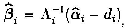

- From linear model theory it is known that under assumptions 1) and 2) α̂i and the residual variance estimator


estimator 



- The estimator β̂ given by equation (7.65) is the customary arithmetic mean estimator


- Consider the sample covariance

- Since


- Consider very small residual variance such that

1, ...b̂m are independent. - In the following, a prediction in the linear mixed model scheme will be described.
- Let Λ be a q × q matrix, and let x be a vector in. Consider the response

Z(x) = (Λ(β+b)+d)T x+ε under the regressor x where the random effect b and the residuals ε are independent of all variables used for parameter estimation. The appropriate predictor for the response is
- Since E[β̂] = β, see equation (7.69)t', we have E[Ẑ(x)]=(Aβ+d)T x = E[Z(x)] and

the prediction variance is
and the prediction error variance is
- Replacing σ2 by


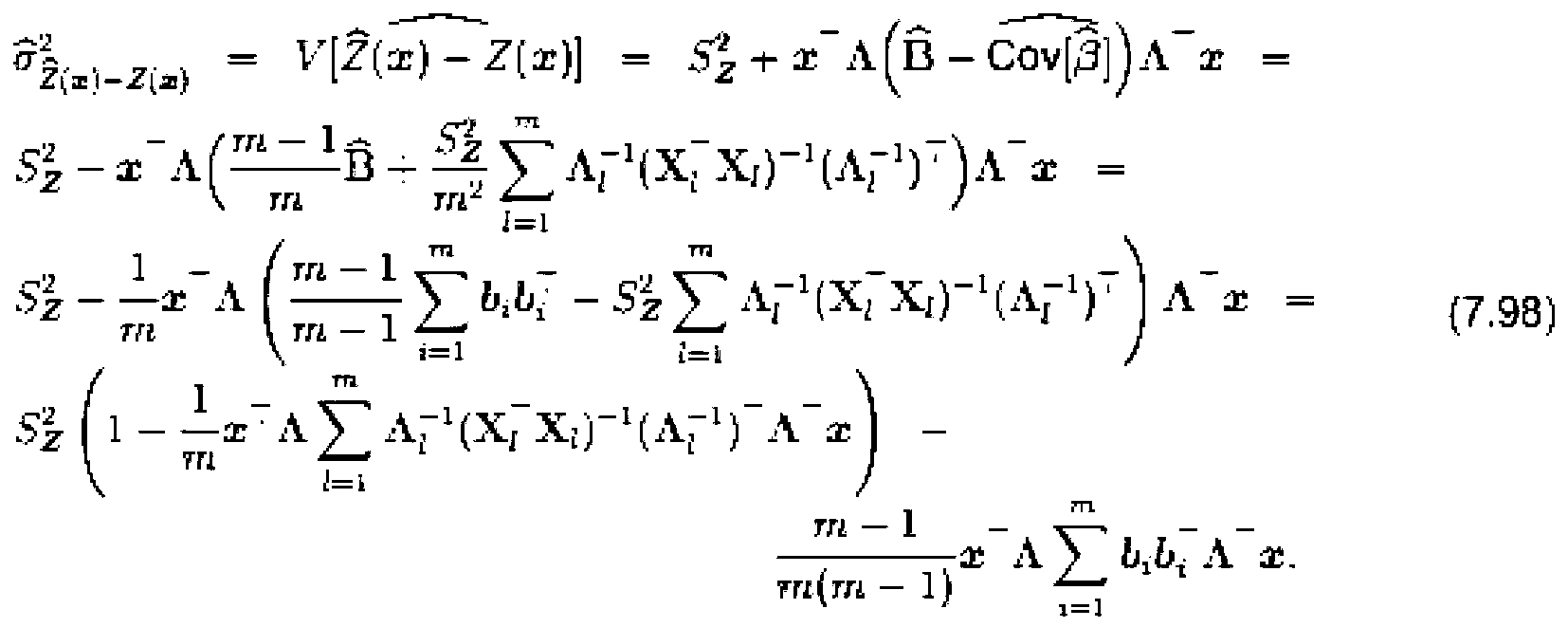
of the prediction error variance
- In the following, a distributional analysis of the estimator of the prediction error variance will be described.
- For the subsequent inferences we consider the assumptions: 1) b 1 has a q-dimensional normal distribution N(0, B). 2) The residual vector εi has a normal distribution N(0, σ2I), i.e., Vi = σ2I. Then the vector b̂ = (b̂ 1,...,b̂ m)T has the m×q-variate normal distribution with E[b̂] = 0, Cov[b̂ i] given by equation (7.83), and with Cov[b̂i ,b̂j ] given by equation (7.85).
- By the above results,

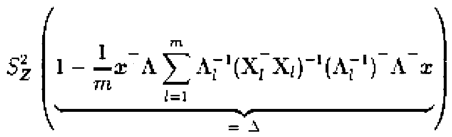
And
are independent. - From the properties of the χ2 distribution we infer

- Under assumptions 1) and 2), we investigate properties of the scalar variable W i=x which appears in the second component of the prediction variance considered above where

- W 1,...,W m have anm-variate joint normal distribution. By (7.70), we have µw i = E[x T Λb̂i ]=0. The variance


- The covariances σ w
i , wj = E[WiWj ] can be inferred from equation (7.85) by using
- By (7.84), we have

- From the theory of multivariate normal distribution we obtain

- Obviously, the second part of equation (7.104) contains the first part as the special case i = j.


- Obviously, equation (7.106) contains equation (7.105) as the special case i = j. From equations (7.105) and (7.106) we obtain

- From (7.98), (7.99), (7.100), (7.107) we obtain

- In the following, an approximate distribution of the estimator of the prediction error variance will be described.
- An approximation of the distribution of the estimator (7.98) of the prediction error variance can be constructed following the known approximation scheme. The distribution of

is approximated by the χ2(v) distribution with the same variance as U v. Hence v is determined from
Hence
- In the following, an approximate prediction interval will be described.
- As described, we consider the assumptions 1) and 2). Additionally, we assume very small residual variance σ2 such that

- By the above results, the prediction error Ẑ(x)-Z(x)=(Λ(β̂-β-b)) Tx and the estimator

mean 0 and variance
- Using the previous result of the previous paragraph with v defined by equation (7.110), the ratio

is approximately distributed by the central t-distribution t(v). Hence approximate bounds for prediction interval for Z(x) are of the form
where z is an appropriate quantile of the central t-distribution t(v). To apply (7.112) in data analysis, the unknown terms in the definition (7.110) of v have to be replaced by estimators:


- In the following, a confidence interval for the forecasting variance will be described.
-
Let 0 < γ < 1, let v = v 0 be defined by equation (7.110) and let z = zχ 2 (v)(γ) be the 100y% quantile of the χ2 distribution χ2(v). We have
- From the above result we have

Hence
is an approximate level γ confidence interval for the forecasting error variance


- In the following, an application of the general mixed model scheme for the analysis of panel life times will be described.
- As to the transformed model as a special case of the general linear mixed model scheme, the previous results can be applied to the analysis of the transformed model equations considered above. The parameters previously introduced may be chosen as follows:


Then


With

- bi,q , q ∈{-1,1}, depends on the parameter β2 in the form

- Where hi,q (β2) is obvious from equation (7.120), or (7.121), respectively.
- In the following, a nonlinear parametrisation will be described.
- Simultaneous parametrisation of h i,-1 and h i,1

- Where


- Let

- Then by (7.121)

- We write

- The estimator of β2 which minimises (7.127) is the OLS estimator of β2 in the nonlinear regression sampling model

- The model (7.128) is the centered version of the model

In the following, a first expansion in β2, with a co,20,l not considered as a function of β2 will be described. - We have

- Hence the linear expansion of h i,-1(β2) around a
point 


- In the following, a first expansion in β2 with a co,20,l considered as a function of β2 will be described.
- We have

- Hence the linear expansion of h i,-1(β2) around a
point 


- In the following, an estimation of β2 will be described.
- The estimator β̂2 should minimise ∑ i∈ Mb̂ i,-1(β2)2. From equation (7.122) we obtain

- Hence

- With h i(β2) ≈ r i+s iβ2, we obtain approximately

- Hence ∑ i∈ Mb̂ i,-1(β2)2 is approximately minimised by

- The result (7.138) can also be obtained in the following manner. With the approximation h i(β2) ≈ r i + s iβ2, we obtain approximately

- Hence the value which minimises ∑ i∈ Mb̂ i,-1(β2)2 is approximately the OLS estimator of β2 in the model

- The OLS estimator is provided by equation (7.138). The approximate validity of the model (7.140) follows from E[b̂i,-1(β2)] We consider the model in the conditional situation given α̂ i , i ∈ M. The design matrix of the model (7.140) is

hence
- Let

variance 

- In the conditional situation, confidence intervals for β̂2 can be calculated in the way familiar from linear regression analysis.
- Forecasts refer to panels stored some time x under non-accelerated conditions at an average temperature c °C, i. e., at T = c + 273:15 K. The corresponding transformation is

- Hence the matrix /\ has to be chosen as

corresponding to whether β0 is assumed to be known or estimated by the method above described, where R = 8:314471 is the gas constant. The forecasting vector x is
- Estimates β̂2 as a of
expansion points 
Fig. 17 , whereingroups 13 and 19 are excluded. - The response predictor (7.94) amounts to

- Or

respectively. The forecast in the untransformed model is
- Where ad is the panel thickness.
- In the following, an estimation of βi0 based on linearised response will be described.
- The subsequent approach is described for general information of the reader. The estimation procedure provided no intuitively reasonable results.
- Consider the transformed model (7.31). For abbreviation, let λ fg = λ free gas . Consider the left-hand side of (7.31) as a function of βi0. We have

- Hence the linear expansion of
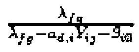


- On the left-hand side of (7.31), replace



- Then we obtain the regression equation

- The previous results can be applied to the analysis of the regression model (7.149). The parameters previously introduced have to be chosen as follows:


- In the following, an estimation of β0 based on maximising forecasts will be described.
- Consider the second mixed model (7.7) with β0 constant over all groups. A least favourable forecast estimator β̂0 can be defined in the following sense: Choose β̂0 which maximises the forecast Ŷ(x) defined by equation (7.145).
- In the following, parameter estimates and prediction will be described.
- As to parameter estimates, we consider the empirical evaluation of the linear mixed model as described. Basis for the evaluation is the data set containing the values of the measurements.
- The following parameters have to be estimated in the order displayed, see also tables 3 and 4:
- 1. The random parameters

- 2. The global parameter β2 representing the activation energy.
- 3. The parameter β0 as a least favourable forecast estimator.
- 4. The components β-1 and β1 of the vector β representing the average initial gas pressure in the panel in units of p 1/2 and the average relative increase in the gas pressure in units of p 1/2, respectively.
- 5. The random parameters
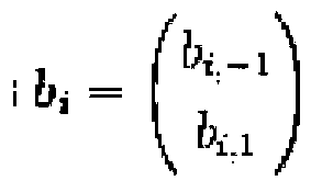
- 6. The variance σ2 representing the measurement uncertainty.
- 7. The covariance matrix B of β representing the uncertainty due to quality differences in the panels.
- For the evaluation the following items have to be taken into account:
1. Groups are identified with panels.
2. Panel 46 is excluded from the analysis due to implausible measurements. Hence a total of 9 panels is included in the analysis.
3. For each panel, only 3 measurings may be available. For the estimation of the parameters β i,-1, β i,1 it is necessary that the measuring points used for the evaluation are equal concerning a time,70,i , the total accelerated exposure time of panel i. The total non-accelerated exposure time x time,20,i,j of panel i until measurement j is the only variable factor. The panels stored in the 20°C-environment are not stored in a 70°C-environment at all such that a time,70,i = 0. These panels do not differ in respect of a time,70,i,, so all the available measuring points can be used for the evaluation, more precisely 3 measuring points for each panel. For the panels which are partly stored in the accelerated 70°C-environment, the accelerated exposure times a time,70,i differ from measuring point to measuring point. The panels are measured in the beginning, then stored in the 70°C-environment and then measured again twice after some time, in which they undergo a 20°C-environment only. Therefore only themeasuring points Table 7: Parameter estimates Estimate Lower confidence limit Upper confidence Unit β-1 0.000403441 - - - β1 0.000604925 - - 1/day β2 42879.7 38320.3 47439.1 J/(mol×K) β0 3.45 - - 10-3W/(m×K)] σ2 0.0000143776 - - - B = Cov[bi ] 
- - - Cov[β̂] 
- - - remark 3, it is impossible to estimate a variance in the measuring of these panels. Therefore the variance is estimated only by the use of the panels stored in the 20°C-environment.
5. Due to expert knowledge the parameter β0 is expected to be in the interval [1; 4]. - Therefore the least favourable case for the parameter β0 is searched for in the interval [1; 4]. Furthermore the two location parameters β0 and β-1 are connected in a negative way: The greater the parameter β0 (location parameter with reference to the activation energy), the lower the estimated value for β-1 (location parameter with reference to the gas pressure). Since a negative value for the parameter β-1 is considered implausible, the parameter β0 is regarded plausible only as long as β-1 is positive.
- Table 5 shows the parameter estimates for the nonlinear mixed model as above described based on the data set containing the values of the measurements. For the estimation, commercially available tools may be used.
- For the validation of the model the parameter estimates based on the measurements are compared with the parameter estimates based on the measurements taken from further measurements.
- For the evaluation the following items have to be taken into account:
- 1. For each panel measuring runs have taken place. Each measuring run is separately analysed, i. e. groups are identified with measurement periods. Particularly, the random parameters βi,1 and βi--1 are estimated for each test run. As a consequence the group index i does not represent different panels as described, but different test runs.
- 2. Test run 13 (=̂ panel 46) is excluded from the analysis due to implausible measurements. No second test run took place for this panel.
- 3. The test run 19 is excluded from the analysis since no second test run took place for the corresponding panel.
- 4. Implausible observations and observations which show unusual behaviour in the beginning of the measuring process are excluded from the analysis.
- 5. To mitigate the potential autocorrelation of measurements taken every five minutes over a period of several days per panel, only each 12th data point is included in the analysis, i. e., the response "thermal conductivity" is regarded once per hour.
- As to prediction we consider the mixed nonlinear model as described. The objective is to predict the response "thermal conductivity", ad,1Y with ad,1 the thickness of panel i, under usage conditions, i. e., for special values of the following two influential factors:
1) Time. This factor is contained in the vector x.
2) Temperature. This factor is contained in the matrix Λ.Table 8: Parameter estimates Estimate Lower confidence limit Upper confidence limit Unit β-1 0.182909 - - βi 0.000873323 - - 1/day β2 39682.8 36450.9 42914.6 J/(mol×K) β0 1.0 - - 10-3W/(m×K) σ 21 21806·10-6 - - - B = Cov b 1. 
- - - Cov β̂. 
- - - - The prediction is based on two components:
- i) point prediction,
- ii) interval prediction.
- The point prediction of the transformed response Z, see equation (7.33), is a prediction of the expected value Ẑ(x)=(Λβ̂+d)T x. Since the model as described uses the transformation

the prediction ad,iŶ for the response "thermal conductivity" can be calculated by retransforming the response Ẑ using the following equation:
- The prediction Ŷ for the response "heat transfer coefficient" can be derived using the following equation, respectively:

- An approximate prediction interval for a future response Z is

where
and z is an appropriate quantile of the central t-distribution. To receive a prediction interval (ad,iYL , ad,iYU ) for the response ad,iY or a prediction interval (YL, YU ) for the response Y, again one can use the retransforming equation (7.154). - The prediction variance, see equation (7.157), is basically formed by
- a) the residual variance σ2 due to measurement uncertainty, estimated by

- b) the variance due the quality differences in the panels, which can be read out of the covariance matrix B, estimated by B̂.
- c) the variance that can partially be controlled by the measurement setup, i. e., the time the panels are stored in the accelerated environment, the overall duration of the experiment, the number of measuring points for each panel, the temperature levels. These experimental factors influence the matrices Λ 1 and X 1 .
- We calculate the prediction for the following values of the influential factors which represent usage conditions:
- 1) Time: 2 years.
- 2) Temperature: 20°C.
- On grounds of the linearised model, the prediction Ẑ(x) by (7.94) and the two-sided prediction limits ZL (x) < ZU (x) by (7.156) at a confidence level of 0.95 are

- Both the point prediction Ẑ(x) and the limits of the prediction interval have to be retransformed by applying equation (7.154). The predicted thermal conductivity and the corresponding prediction limits given in W/(mK) at a confidence level of y = 0:95 are

- To illustrate the influence of the different components of the prediction variance, the prediction variance and its components are calculated. Using the above conditions for the prediction and the estimated parameter values from table 7, the following values are obtained:



- These results show that the variance 0.0168818, which is basically due to quality differences in the panels, dominates the variance

- As to the experimental design of experiments for life time prediction, the analysis is based on the mixed model as described. The objective is to ensure a prediction of future values which is as exact as possible without neglecting certain external restrictions. The empirical basis for the design study is the data set containing the values of the measurements.
- The following questions are considered in this context:
- 1. How many different panels m have to be included in the experiment?
- 2. How should the panels be divided into two groups of sizes m1 , m2 , with m 1 panels being stored in the low-temperature-environment and m 2 panels being stored in the accelerated-temperature-environment?
- 3. How much time should at least be scheduled for the whole experimental process?
- 4. How should the storing environments be chosen, more precisely, which two temperature levels should be chosen for the panels to be stored in?
- 5. How long should the panels of the accelerated temperature group be stored in the accelerated environment before being stored in the lower temperature environment and be measured a few times during that period?
- 6. How often should each panel be measured in the course of the whole measuring period?
- The precision in the prediction is reflected in the length of the prediction interval (7.156). The lower the length of the prediction interval, the more exact a future observation can be predicted. The crucial component of the prediction interval is the variance of the prediction, see formula (7.98). The objective of an ideal construction of an experimental design is therefore minimising the length of the prediction interval, see formula (7.112).
- However, due to the nature of the mixed model, the prediction interval (7.98) cannot be used to answer each of the questions mentioned above in the same way.
- The experimental design aims at minimising one of the following functions of the prediction variance keeping in mind the above remarks. The prediction is calculated for panels stored for 2 years in a 20°C-environment at a confidence level of 95%:
- Length of the prediction interval:

- Squared length of the prediction interval:

This term is mainly influenced by the differences in panel quality and can basically be reduced by increasing the number m of testing panels. - The part of the variance of the prediction which is basically influenced by the measurement setup. We consider the following terms:


- In the above cases z is an appropriate quantile of the t-distribution. For the construction of the experimental design the following estimated values derived from the original data set have to be used, see table 7:
- The estimated variance,

- The estimated value β̂2 for the parameter β2.
- The estimated worst case value for the parameter β0, β̂0.
- The estimated components β̂-1 and β̂1 of the vector β.
- The covariance matrix β̂ of b.
- The parameter β2 depends on the random parameters α i0 and α i1, i = l,..., m, and can only be estimated after the estimation of these parameters. Therefore, and since the estimation of β2 differs with the experimental design used, the following conservative approach is taken: The prediction interval is calculated with the value for β2 taken from its confidence interval which maximises the length of the two-sided prediction interval.
- Regarding the construction of the experimental design the following approach is taken:
- 1. For each measurement setup with a prescribed number of testing panels, temperatures and storing time of the panels in the available environments, at least 10 000 sets of random values α i0, α i1 are simulated using the information about their distribution, E[α̂0], E[α̂1] and Cov[α̂ i ]. see equations (7.68) and (7.77).
- 2. For each simulated set, an estimation and confidence interval for the parameter β2 is calculated. The level of the confidence interval is chosen in a way, so that the uncertainty that comes with the estimation of β2 and the uncertainty in the calculation of the prediction interval in total is maximally the prescribed maximum error 1 - γ. A prescribed level γ in the final prediction interval is obtained via the Bonferroni inequality by choosing partial levels γi = 0.5(1+γ) for the confidence level for β2 and for the prediction interval depending on β2.
- 3. For each value of β2 in its confidence interval the future prediction along with its prediction interval is calculated.
- 4. From all possible prediction intervals the one selected for the analysed measurement setup is the one which maximises the length of the prediction interval.
- 5. The results achieved by simulating 10 000 sets of random values for α i0, α i1 are averaged. These mean values are used to compare different measurement setups.
- As to selection of measuring points, the mixed model analysis estimates some parameters for each panel separately, in particular the residual variance (measurement variance). At least three measuring points are necessary to secure the possibility of estimating the measuring variance for each panel. To exceed the unreliable minimum, it is advised to measure each panel at least four times in the course of the measuring period. Since the measuring variance is regarded rather small in general, four measuring points are assumed to be enough. It is advised that the measuring points are arranged in equal distances making use of the whole available measurement period.
- As to the choice of the number of testing panels, since in the case at hand the uncertainty in the prediction is mainly influenced by the differences in quality of the panels, the accuracy of the prediction can be improved most by increasing the number of testing panels.
-
Fig. 18 shows the length LU - LL of the prediction interval for the transformed values, the contribution Φ of the measurement setup to the prediction variance of the transformed values and the length of the prediction interval for the thermal conductivity (unit: W/(mK)) as a function of the number of testing panels. The calculation is based on the following measurement setup: - Temperature levels: 25°C, 70°C.
- Storage time in the 70°C-environment: 60 days.
- Length of the overall measuring period: 120 days.
- Times of measuring for panels stored in a 25°C-environment in days from the beginning: 0, 40, 80, 120 days.
- Times of measuring for panels stored in a 70°C-environment in days from the end of the storage time in the 70°C-environment: 0, 20, 40, 60 days.
- The length of the prediction interval is calculated for the following divisions of the panels into the two temperature groups:
- a)

- b) m 1 = 2m 2: Only half as many panels, m 2, are stored in a 70°C-environment as are stored in a 25°C-environment, m 1.
-
Fig. 19 shows that a huge improvement in prediction accuracy can be achieved by increasing the number of testing panels involved in the experiment up to a number of about 24. Only a minor improvement can be observed when including more than about 24 testing panels in the experiment. To assess the influence of the temperatures the panels are stored in, we compare the term Φ for the two cases m 1 = m 2 and m 1 = 2m 2. Φ reveals an advantage for the case m 1 = m 2 compared to the case m 1 = 2m 2, i. e., it seems to be better to store as many panels in the 25°C-environment as in the 70°C-environment than twice as many. -
Fig. 20 shows the squared length (LU - LL )2 of the prediction interval and the termΦ , see equation (8.4), with the intention of comparing the two quantities. It is obvious thatΦ , which contains the influences of the experimental design, is comparably small in comparison to (LU - LL )2. - As to the choice of the length of the measuring period the length of the overall measuring period mainly influences the matrices XI, and indirectly the matrices A and Λ 1 , l = 1,..., m, in the prediction variance (7.157). Therefore, the decision on the total length of the measuring period should be based on the minimisation of the term Φ, see equation (8.3). Note that Φ is comparably small in the case at hand. Compared to the number of testing panels it does not influence the accuracy of the prediction a lot.
Fig. 21 shows the component Φ of the prediction variance as a function of the length of the overall experimental time. The calculation is based on the following measurement setup: - Temperature levels: 25°C, 70°C.
- Number of panels in each temperature group: 6, i. e. a total of 12 panels.
- Storage time in the 70°C-environment: 60 days.
- Varying the length of the overall experimental time means the following times of measuring:
- Times of measuring for panels stored in a 25°C-environment: Four equally distanced measuring points over the entire measuring period.
- Times of measuring for panels stored in a 70°C-environment: Four equally distanced measuring points over the measuring period beginning after 60 days of storing the panels in the 70°C-environment.
-
Figure 19 shows that strong improvement in Φ can be achieved when choosing at least 150 days for the total length of the measuring period. The length of the prediction interval in units W/(mK) decreases only little if the measuring period is extended beyond 150 days. - As to the choice of the storing environments, the choice of the storing environments for the panels, i. e., the two temperature levels the panels are faced with during the whole experimental process, influences the matrices X1 Λ and Λ1, l = 1,..., m, in the prediction variance (7.157). Therefore the decision on the temperature levels for the storing environments for the panels during the experimental process should be based on the minimisation of the term Φ, see equation (8.3). For reasons of simplicity, the lower of the two temperature levels should be approximately room temperature, i. e., between about 10 and 25°C. Since applications have shown that a storage temperature of more than about 70°C might cause a destruction of the panels in a short time, storage temperatures of more than about 80°C are not considered in the analysis. For the analysis, the non-accelerated temperature is prescribed at 25°C, which is considered to be an upper bound for temperature stress in domestic applications.
-
Figure 20 shows the component Φ, see equation (8.3), of the prediction variance as a function of the accelerated temperature level in °C for the three following cases: - a) Storage time in the 70°C-environment: 60 days. Length of the measuring period: 120 days.
- b) Storage time in the 70°C-environment: 40 days. Length of the measuring period: 120 days.
- c) Storage time in the 70°C-environment: 40 days. Length of the measuring period: 100 days.
- The other quantities are kept constant for the calculation on the following values:
- Temperature level of the low temperature: 25°C.
- Number of panels in each temperature group: 6, i.e., a total of 12 panels.
- Times of measuring for panels stored in a 25°C-environment in days from the beginning: 0, 40, 80, 120 days.
- Times of measuring for panels stored in a 70°C-environment in days from the end of the storage time in the 70°C-environment: Four equally distanced measuring points over the measuring period beginning after the storing time in the 70°C-environment.
- The first plot in
Fig. 20 which represents the results for a storage time in the 70°C-environment of 60 days reveals a minimum in Φ at an accelerated temperature of about 70°C. The second plot representing the results for a storage time in the 70°C-environment of 40 days reveals a minimum in Φ at an accelerated temperature of about 80°C. Both plots are based on a measuring period of 120 days. The third plot shows the results for a storage time in the 70°C-environment of 40 days with a measuring period of only 100 days. The minimum in Φ can be observed at an accelerated temperature of 80°C as well. - Both the time the panels are stored in the accelerated environment as well as the accelerated temperature itself are acceleration factors in the experiments. Hence from
Fig. 20 it can be concluded that if panels are stored less time in the accelerated environment, the lower acceleration effect can be compensated if in return the accelerated temperature level is increased. Nevertheless to choose the accelerated temperature above a certain level can be disadvantageous. Furthermore reducing the length of the whole measuring period causes worse results in the precision of the prediction. - As to the choice of the storing time in the accelerated environment, the choice of the storing time of panels in the accelerated environment influences on the matrices X1, Λ and Λ1,l = 1,...., m 1, in the prediction variance (7.157). Therefore the decision on the length of the accelerated storing period should be based on the minimisation of the term Φ, see equation (8.3).
-
Fig. 20 shows the component Φ, see equation (8.3), of the prediction variance as a function of the time the panels are stored in the accelerated environment in days. The calculation is based on the following measurement setup: - Temperature levels: 25°C, 70°C.
- Number of panels in each temperature group: 6, i. e., a total of 12 panels.
- Length of the overall measuring period: 120 days.
- Times of measuring for panels stored in a 25°C-environment in days from the beginning: 0, 40, 80, 120 days.
- Times of measuring for panels stored in a 70°C-environment in days: Four equally distanced measuring points over the measuring period beginning after the storing time in the 70°C-environment.
-
Fig. 20 shows a minimum in Φ at a storing time in the 70°C-environment of about 55 days. Hence under the above measurement setup.Fig. 20 suggests that optimally panels should be stored in a 70°C-environment for almost two months before being measured 4 times under room temperature. -
Fig. 21 shows Φ as a function of the accelerated temperature level. -
Fig. 22 shows Φ as a function of the storage time of the panels in the accelerated environment in days. - As to the operating instructions, the choice of the experimental design depends on the amount of the variation due to differences in the panel quality. Therefore first of all examinations should be taken on how much the panel-to-panel variation influences the accuracy in the prediction in comparison to the other factors determining the experimental design.
- In the following, the choice of the experimental factors and their levels will be described.
- As to the choice of the length of the measuring period, the accuracy in the prediction can be improved by extending the measuring period. A measuring period of at least 150 days should bring reasonable results in the prediction. The measurements on panels which are stored under approximately room temperature should begin with the start of the experiment. Panels which are stored in an accelerated environment should first remain in that environment for a prescribed time, and should afterwards being measured. If the panel-to-panel variation is comparably high, a shortening of the measuring period might be justifiable if in return the number of panels is increased.
- On the contrary, if in future experiments the panel-to-panel variation is comparably small, extending the length of the measuring period might have greater influence on the accuracy of the prediction and might be worth considering.
- As to the selection of measuring points, each panel may be measured 4 times. The measuring points should be equally distributed over the entire measuring period. I. e., for panels stored at room temperature, the first measuring point is the starting time of the experiment, and for panels stored under in an accelerated environment, the first measuring point is the time point right after the end of the accelerated storing period. For both groups of panels, the last measuring point is at the end of the experimental period.
- As to the choice of the storing time in the accelerated environment panels subject to accelerated exposure may remain in the accelerated environment over almost two months before starting the measurement period.
- As to the choice of the storing environments, two temperature levels should be chosen in which the panels are stored during the experiment. Partly the panels are recommended to be stored in an environment of about 25°C which is approximately room temperature. The remaining panels should be stored in an environment of about 70°C if the storing time in the accelerated environment is chosen to be 60 days. If this period is shortened, the acceleration effect can nevertheless be achieved by increasing the accelerated temperature.
- As to the choice of the number of testing panels, a number of at least 24 testing panels are recommended to be included in the experiment.
- The panels can be divided into to equally sized groups: one group being stored in a 25°C-environment, and the other in a 70°C-environment. Whether to increase the number of testing panels or rather to increase the length of the measuring period depends on what is the decisive factor for the prediction variance: panel-to-panel variation or the measurement-to-measurement variation.
- As to the prediction of the proportion of nonconforming items, to predict the proportion of nonconforming items, the point prediction Ẑ(x) as well as the two-sided prediction interval

have to be examined. By a suitable choice of the quantile


I. e., the probability that the real value for the response Z(x) lies in the interval Bx is γ. - To be able to make conclusions in units of thermal conductivity, it is necessary to retransform the values Ẑ(x), ZL (x), and ZU (x). A prediction ad,iŶ(x) for the thermal conductivity as well as a prediction interval (ad,iYL (x), ad,iYU (x)) can be derived by using the transforming equation

- The unknown parameter β0 has to be replaced by the estimator β̂0 from the actual experiment. The estimator is determined as described above.
- As to the prediction based on prescribed confidence levels 0.99 and 0.95 for the prediction is prescribed, we consider the prescribed confidence levels 0.99 and 0.95 in the following.
- Consider the prediction interval (ad,iYL (x), ad,iYU (x)) for a prescribed confidence level of 0:99. If the upper bound ad,iYU (x) does not exceed a critical value c for the thermal conductivity, it can be argued, that in the long run not more than (1 - 0:99) · 100% = 1 % of the panels are expected to exceed c in the thermal conductivity.
- If the upper bound of the prediction interval for the given confidence level 0:99 is higher than the critical value c, the prediction interval should be calculated for a confidence level of 0:95. If the upper bound of the prediction interval for a confidence level of 0:95 lies below c, one can conclude that in the long run less than (1-0:95) · 100% = 5% of the panels are expected to exceed the critical value c.
- As to the prediction based on random confidence level, the approach to predict the proportion of nonconforming items where the confidence level is not prescribed but random may be deployed.
- The following two cases have to be distinguished:
- 1. ad,iŶ(x) < c, i.e.., the point prediction ad,iŶ(x) lies below the critical value c. In this case, consider the upper bound ad,iYU (x) of the prediction interval. Determine γ in a way, that

which requires a suitable choice of
- 2. ad,iŶL (x) > c, i.e.,., the point prediction ad,iŶ(x) lies above the critical value c. In this case, consider the lower bound ad,iYL (x) of the prediction interval. Determine γ in a way, that

which requires a suitable choice of
- As to the prediction based on one-sided prediction intervals, the preceding analysis is based on two-sided prediction intervals for the thermal conductivity. A different approach to decide on how many panels exceed the critical values 0.008 W/(m· K) for 2 years and 0.015 W/(m· K) for 10 years in the thermal conductivity, would be to consider the one-sided prediction interval with an upper bound:

and the retransformed interval
respectively. If the quantile z is chosen as z = z (γ), a prescribed forecasting confidence level γ can be achieved. If the upper bound ad,iY̅U (x) is below the critical value c for the thermal conductivity it can be concluded that in the long run not more than (1 - γ) · 100% of the panels are expected to exceed c. Otherwise no conclusion is possible, i. e. the percentage of the panels exceeding the critical values cannot be estimated below 100%.
This approach allows to decide what percentage of the panels exceed the critical value at the utmost while ensuring a higher confidence level for the prediction than in the case of a two-sided prediction interval. Nevertheless, to ensure the possibility of drawing a conclusion, this method is only recommended if the predicted response is far below the critical value c. - In the case at hand, the basis for the investigations were measurements taken on highly degrading panels with high panel-to-panel variation that are not suitable and cannot be used for the intended purpose. Since the critical values for the thermal conductivity are not far from the point prediction, no conclusion would be possible in many cases if one-sided prediction intervals were used. Therefore, the investigations concentrated on two-sided prediction intervals which allow to estimate an interval with upper and lower bound in which the future observations lie with a high probability. Also, the two-sided interval allows to compare the accuracy of the prediction by means of the length of the prediction interval, and is suitable especially for the construction of an experimental design.
- For future investigations, other panels with lower degradation rates and lower panel-to-panel variation are expected. In this case, one-sided prediction intervals with an upper bound will probably be the appropriate method to find an upper bound for the percentage of nonconforming panels.
- According to some embodiments, the following steps were basically taken:
- 1. A standard fixed effects nonlinear regression model was built using the relation between the gas pressure and the thermal conductivity. The problem was that panel-to-panel variation could not be taken account of by the fixed effects model.
- 2. A mixed nonlinear regression model was constructed including random parameters that model panel-to-panel variation.
- 3. The mixed nonlinear regression model was transformed to a linear model.
- 4. Regression parameters were estimated based on the transformed mixed model.
- 5. The statistical inference theory for a linear mixed model was derived.
- 6. The general mixed model scheme was applied to the analysis of panel life times.
- 7. An experimental design on the basis of a mixed regression model was developed.
- The initial data basis were measurings. By this means increases in the thermal conductivity could be expected to be measured accurately. At the same time, further measurings were taken for control purposes. In the course of the project, while deriving an optimal experimental design, it was realised that it would be necessary to include a high number of testing panels in future experiments to make precise predictions for the thermal conductivity.
-
- 101
- measuring
- 103
- measuring
- 107
- executing
- 201-215
- method steps
- 217
- fitting the regression model
- 219
- executing the regression model
Claims (18)
- Method for predicting a physical characteristic of vacuum insulation panels of a certain type, the method comprising:measuring (101) a plurality of physical quantities associated with the vacuum insulation panels at distinct time instants;measuring (103) values of the physical characteristic at the distinct time instants;fitting (105) a parametric regression model with the measured physical quantities as regression parameters to predict the measured values of the physical characteristic at the distinct time instants using the parametric regression model;andexecuting (107) the parametric regression model to predict the physical characteristic at a future time instant.
- The method of claim 1, wherein the parametric regression model is executed and/or fitted by a computer.
- The method of claim 1 or 2, wherein the parametric regression model is a non-linear regression model, in particular a mixed non-linear regression model.
- The method of anyone of the preceding claims, wherein the values of the physical characteristic and the plurality of physical quantities are measured at three distinct time instants, in particular only at three distinct time instants.
- The method of anyone of the preceding claims, wherein the physical characteristic is a least one of: thermal conductivity, internal gas pressure, weight.
- The method of anyone of the preceding claims, wherein the measured physical quantities are at least one of the following physical quantities: temperature, elapsed time during which a vacuum insulation panel was exposed to a certain test condition, in particular to a certain temperature, geometry of a vacuum insulation panel, in particular a sealing length or a surface area or a volume of a kernel of a vacuum insulation panel or a thickness of a vacuum insulation panel, a mass of a vacuum insulation panel, a relative mass increase of a vacuum insulation panel.
- The method of anyone of the preceding claims, wherein the step of fitting (105) of the parametric regression model comprises determining regression coefficients of the parametric regression model.
- The method of anyone of the preceding claims, further comprising determining the distinct time instants for measurements.
- The method of anyone of the preceding claims, further comprising determining a number of vacuum insulation panels of the same type for measurements.
- The method of anyone of the preceding claims, further comprising determining a total measurement time of the measurements.
- The method of anyone of the preceding claims, further comprising determining environmental conditions, in particular temperatures, to which to expose at least one vacuum insulation panel.
- The method of claim 11, further comprising determining an exposure time.
- The method of anyone of the preceding claims, further comprising determining a number of measurements repetitions.
- The method of anyone of the preceding claims, wherein the vacuum insulation panel of the same type comprise a panel core, in particular a fiber panel core.
- The method of anyone of the preceding claims, wherein the parametric regression model is one of the following parametric regression models


with Y denoting values of the physical characteristic, β1 - β4 denoting regression coefficients, x1 - x4 denoting measured values of the physical characteristic and ε denoting an error. - The method of anyone of the preceding claims 1 to 14, wherein the parametric regression model is described by a nonlinear function

with i denoting an group index of vacuum insulation panels, j denoting a measurement index, Yij denoting a measured value of the physical characteristic at i, j, xij denoting measured values of the physical characteristic, ai denoting a level of a measured physical characteristic, β denoting a regression coefficient, bi denoting a random deviation of a vacuum insulation panel, and εi,j denoting an error. - The method of anyone of the preceding claims, wherein the predicting the physical characteristic of the vacuum insulation panels comprises predicting a number of vacuum insulation panels having a certain value of the physical characteristic or having a value of the physical characteristic below or above a threshold.
- The method of anyone of the preceding claims, wherein the predicting the physical characteristic of the vacuum insulation panels comprises predicting a change of the physical characteristic over time.
Priority Applications (1)
| Application Number | Priority Date | Filing Date | Title |
|---|---|---|---|
| EP11189757.5A EP2594924B1 (en) | 2011-11-18 | 2011-11-18 | Method for predicting a physical characteristic of vacuum insulation panels |
Applications Claiming Priority (1)
| Application Number | Priority Date | Filing Date | Title |
|---|---|---|---|
| EP11189757.5A EP2594924B1 (en) | 2011-11-18 | 2011-11-18 | Method for predicting a physical characteristic of vacuum insulation panels |
Publications (2)
| Publication Number | Publication Date |
|---|---|
| EP2594924A1 true EP2594924A1 (en) | 2013-05-22 |
| EP2594924B1 EP2594924B1 (en) | 2017-08-23 |
Family
ID=45033836
Family Applications (1)
| Application Number | Title | Priority Date | Filing Date |
|---|---|---|---|
| EP11189757.5A Active EP2594924B1 (en) | 2011-11-18 | 2011-11-18 | Method for predicting a physical characteristic of vacuum insulation panels |
Country Status (1)
| Country | Link |
|---|---|
| EP (1) | EP2594924B1 (en) |
Cited By (3)
| Publication number | Priority date | Publication date | Assignee | Title |
|---|---|---|---|---|
| CN115289404A (en) * | 2022-07-25 | 2022-11-04 | 中国石油化工股份有限公司 | A service life prediction method, storage medium and equipment of a pipeline thermal insulation material |
| JP2023157800A (en) * | 2022-04-15 | 2023-10-26 | パナソニックIpマネジメント株式会社 | Generation method, generation device, and program |
| CN118242633A (en) * | 2024-05-28 | 2024-06-25 | 内江市检验检测中心 | A method for online monitoring of stress intensity of pressure-bearing components outside a boiler |
-
2011
- 2011-11-18 EP EP11189757.5A patent/EP2594924B1/en active Active
Non-Patent Citations (4)
| Title |
|---|
| BRUNNER ET AL: "In situ performance assessment of vacuum insulation panels in a flat roof construction", VACUUM, PERGAMON PRESS, GB, vol. 82, no. 7, 21 December 2007 (2007-12-21), pages 700 - 707, XP022502934, ISSN: 0042-207X, DOI: 10.1016/J.VACUUM.2007.10.016 * |
| FRICKE ET AL: "Vacuum insulation panels-From research to market", VACUUM, PERGAMON PRESS, GB, vol. 82, no. 7, 20 December 2007 (2007-12-20), pages 680 - 690, XP022502932, ISSN: 0042-207X, DOI: 10.1016/J.VACUUM.2007.10.014 * |
| SCHWAB H ET AL: "Prediction of service life for vacuum insulation panels with fumed silica kernel and foil cover", JOURNAL OF THERMAL ENVELOPE AND BUILDING SCIENCE APRIL 2005 SAGE PUBLICATIONS LTD GB, vol. 28, no. 4, April 2005 (2005-04-01), pages 357 - 374, XP008148804, DOI: 10.1177/1097196305051894 * |
| WEN Y ET AL: "Service life evaluation of FG-type vacuum insulation panel", ZHENKONG KEXUE YU JISHU XUEBAO/JOURNAL OF VACUUM SCIENCE AND TECHNOLOGY FEBRUARY 2011 SCIENCE PRESS CHN, vol. 31, no. 1, February 2011 (2011-02-01), pages 110 - 113, XP008148862, DOI: 10.3969/J.ISSN.1672-7126.2011.01.22 * |
Cited By (3)
| Publication number | Priority date | Publication date | Assignee | Title |
|---|---|---|---|---|
| JP2023157800A (en) * | 2022-04-15 | 2023-10-26 | パナソニックIpマネジメント株式会社 | Generation method, generation device, and program |
| CN115289404A (en) * | 2022-07-25 | 2022-11-04 | 中国石油化工股份有限公司 | A service life prediction method, storage medium and equipment of a pipeline thermal insulation material |
| CN118242633A (en) * | 2024-05-28 | 2024-06-25 | 内江市检验检测中心 | A method for online monitoring of stress intensity of pressure-bearing components outside a boiler |
Also Published As
| Publication number | Publication date |
|---|---|
| EP2594924B1 (en) | 2017-08-23 |
Similar Documents
| Publication | Publication Date | Title |
|---|---|---|
| Lu et al. | Uncertainty evaluation of humidity sensors calibrated by saturated salt solutions | |
| EP2594924B1 (en) | Method for predicting a physical characteristic of vacuum insulation panels | |
| Yoon et al. | Strategies for virtual in-situ sensor calibration in building energy systems | |
| CN112504512B (en) | Temperature sensor accuracy self-detection and self-calibration method, electronic device, and storage medium | |
| US20130253873A1 (en) | Calibration of flowmeters | |
| Cheng et al. | Air change rate measurements using tracer gas carbon dioxide from dry ice | |
| Schofield | Vaccine stability study design and analysis to support product licensure | |
| US20190078799A1 (en) | Method and device for determining the air change rate of a room or building | |
| Wang et al. | Propagation of uncertainties in measurements using generalized inference | |
| Jack et al. | Quantifying the effect of window opening on the measured heat loss of a test house | |
| Schibig et al. | Experiments with CO 2-in-air reference gases in high-pressure aluminum cylinders | |
| Cocci et al. | A comprehensive Bayesian framework for the development, validation and uncertainty quantification of thermal-hydraulic models | |
| US20160018372A1 (en) | Method for operating a measuring site | |
| KR101940037B1 (en) | Portable gas detector and re-calibration method thereof | |
| EP3234563B1 (en) | Method for calibrating a device for measuring the concentration of creatinine | |
| White et al. | δ13C and δ18O heterogeneities in carbonates: Nonlinear mixing in the application of dual‐carbonate‐clumped isotope thermometer | |
| Belanger et al. | The impact of aging on the effective thermal conductivity of foam insulation: A simulation investigation using laboratory characterization data | |
| Tijskens et al. | Using convolutional neural networks for hygrothermal predictions to extrapolate to other external climates | |
| Doma et al. | Investigating the Thermal Performance of Canadian Houses Using Smart Thermostat Data. | |
| Bell et al. | A roadmap for humidity and moisture measurement | |
| Hernandez et al. | Non linear state space modelling of a PEMFC | |
| CN223377285U (en) | Standard release container and gas release rate standard determining system | |
| Gureyev et al. | High accuracy semiautomatic calibration of industrial RTDs | |
| Fossa et al. | Use and calibration of capacitive RH sensors for the hygrometric control of the CMS tracker | |
| Yan et al. | Optimization of accelerated destructive degradation testing of cementitious materials for their performances qualification under aggressive environments: the case of carbonation |
Legal Events
| Date | Code | Title | Description |
|---|---|---|---|
| PUAI | Public reference made under article 153(3) epc to a published international application that has entered the european phase |
Free format text: ORIGINAL CODE: 0009012 |
|
| AK | Designated contracting states |
Kind code of ref document: A1 Designated state(s): AL AT BE BG CH CY CZ DE DK EE ES FI FR GB GR HR HU IE IS IT LI LT LU LV MC MK MT NL NO PL PT RO RS SE SI SK SM TR |
|
| AX | Request for extension of the european patent |
Extension state: BA ME |
|
| 17P | Request for examination filed |
Effective date: 20131122 |
|
| RBV | Designated contracting states (corrected) |
Designated state(s): AL AT BE BG CH CY CZ DE DK EE ES FI FR GB GR HR HU IE IS IT LI LT LU LV MC MK MT NL NO PL PT RO RS SE SI SK SM TR |
|
| 17Q | First examination report despatched |
Effective date: 20131216 |
|
| RAP1 | Party data changed (applicant data changed or rights of an application transferred) |
Owner name: BSH HAUSGERAETE GMBH |
|
| GRAP | Despatch of communication of intention to grant a patent |
Free format text: ORIGINAL CODE: EPIDOSNIGR1 |
|
| INTG | Intention to grant announced |
Effective date: 20170411 |
|
| GRAS | Grant fee paid |
Free format text: ORIGINAL CODE: EPIDOSNIGR3 |
|
| GRAA | (expected) grant |
Free format text: ORIGINAL CODE: 0009210 |
|
| AK | Designated contracting states |
Kind code of ref document: B1 Designated state(s): AL AT BE BG CH CY CZ DE DK EE ES FI FR GB GR HR HU IE IS IT LI LT LU LV MC MK MT NL NO PL PT RO RS SE SI SK SM TR |
|
| REG | Reference to a national code |
Ref country code: GB Ref legal event code: FG4D |
|
| REG | Reference to a national code |
Ref country code: CH Ref legal event code: EP |
|
| REG | Reference to a national code |
Ref country code: AT Ref legal event code: REF Ref document number: 921885 Country of ref document: AT Kind code of ref document: T Effective date: 20170915 |
|
| REG | Reference to a national code |
Ref country code: IE Ref legal event code: FG4D |
|
| REG | Reference to a national code |
Ref country code: DE Ref legal event code: R096 Ref document number: 602011040799 Country of ref document: DE |
|
| REG | Reference to a national code |
Ref country code: NL Ref legal event code: MP Effective date: 20170823 |
|
| REG | Reference to a national code |
Ref country code: LT Ref legal event code: MG4D |
|
| REG | Reference to a national code |
Ref country code: AT Ref legal event code: MK05 Ref document number: 921885 Country of ref document: AT Kind code of ref document: T Effective date: 20170823 |
|
| PG25 | Lapsed in a contracting state [announced via postgrant information from national office to epo] |
Ref country code: NO Free format text: LAPSE BECAUSE OF FAILURE TO SUBMIT A TRANSLATION OF THE DESCRIPTION OR TO PAY THE FEE WITHIN THE PRESCRIBED TIME-LIMIT Effective date: 20171123 Ref country code: HR Free format text: LAPSE BECAUSE OF FAILURE TO SUBMIT A TRANSLATION OF THE DESCRIPTION OR TO PAY THE FEE WITHIN THE PRESCRIBED TIME-LIMIT Effective date: 20170823 Ref country code: FI Free format text: LAPSE BECAUSE OF FAILURE TO SUBMIT A TRANSLATION OF THE DESCRIPTION OR TO PAY THE FEE WITHIN THE PRESCRIBED TIME-LIMIT Effective date: 20170823 Ref country code: AT Free format text: LAPSE BECAUSE OF FAILURE TO SUBMIT A TRANSLATION OF THE DESCRIPTION OR TO PAY THE FEE WITHIN THE PRESCRIBED TIME-LIMIT Effective date: 20170823 Ref country code: SE Free format text: LAPSE BECAUSE OF FAILURE TO SUBMIT A TRANSLATION OF THE DESCRIPTION OR TO PAY THE FEE WITHIN THE PRESCRIBED TIME-LIMIT Effective date: 20170823 Ref country code: LT Free format text: LAPSE BECAUSE OF FAILURE TO SUBMIT A TRANSLATION OF THE DESCRIPTION OR TO PAY THE FEE WITHIN THE PRESCRIBED TIME-LIMIT Effective date: 20170823 Ref country code: NL Free format text: LAPSE BECAUSE OF FAILURE TO SUBMIT A TRANSLATION OF THE DESCRIPTION OR TO PAY THE FEE WITHIN THE PRESCRIBED TIME-LIMIT Effective date: 20170823 |
|
| PG25 | Lapsed in a contracting state [announced via postgrant information from national office to epo] |
Ref country code: RS Free format text: LAPSE BECAUSE OF FAILURE TO SUBMIT A TRANSLATION OF THE DESCRIPTION OR TO PAY THE FEE WITHIN THE PRESCRIBED TIME-LIMIT Effective date: 20170823 Ref country code: PL Free format text: LAPSE BECAUSE OF FAILURE TO SUBMIT A TRANSLATION OF THE DESCRIPTION OR TO PAY THE FEE WITHIN THE PRESCRIBED TIME-LIMIT Effective date: 20170823 Ref country code: ES Free format text: LAPSE BECAUSE OF FAILURE TO SUBMIT A TRANSLATION OF THE DESCRIPTION OR TO PAY THE FEE WITHIN THE PRESCRIBED TIME-LIMIT Effective date: 20170823 Ref country code: IS Free format text: LAPSE BECAUSE OF FAILURE TO SUBMIT A TRANSLATION OF THE DESCRIPTION OR TO PAY THE FEE WITHIN THE PRESCRIBED TIME-LIMIT Effective date: 20171223 Ref country code: GR Free format text: LAPSE BECAUSE OF FAILURE TO SUBMIT A TRANSLATION OF THE DESCRIPTION OR TO PAY THE FEE WITHIN THE PRESCRIBED TIME-LIMIT Effective date: 20171124 Ref country code: LV Free format text: LAPSE BECAUSE OF FAILURE TO SUBMIT A TRANSLATION OF THE DESCRIPTION OR TO PAY THE FEE WITHIN THE PRESCRIBED TIME-LIMIT Effective date: 20170823 Ref country code: BG Free format text: LAPSE BECAUSE OF FAILURE TO SUBMIT A TRANSLATION OF THE DESCRIPTION OR TO PAY THE FEE WITHIN THE PRESCRIBED TIME-LIMIT Effective date: 20171123 |
|
| PG25 | Lapsed in a contracting state [announced via postgrant information from national office to epo] |
Ref country code: RO Free format text: LAPSE BECAUSE OF FAILURE TO SUBMIT A TRANSLATION OF THE DESCRIPTION OR TO PAY THE FEE WITHIN THE PRESCRIBED TIME-LIMIT Effective date: 20170823 Ref country code: DK Free format text: LAPSE BECAUSE OF FAILURE TO SUBMIT A TRANSLATION OF THE DESCRIPTION OR TO PAY THE FEE WITHIN THE PRESCRIBED TIME-LIMIT Effective date: 20170823 Ref country code: CZ Free format text: LAPSE BECAUSE OF FAILURE TO SUBMIT A TRANSLATION OF THE DESCRIPTION OR TO PAY THE FEE WITHIN THE PRESCRIBED TIME-LIMIT Effective date: 20170823 |
|
| REG | Reference to a national code |
Ref country code: DE Ref legal event code: R097 Ref document number: 602011040799 Country of ref document: DE |
|
| PG25 | Lapsed in a contracting state [announced via postgrant information from national office to epo] |
Ref country code: SK Free format text: LAPSE BECAUSE OF FAILURE TO SUBMIT A TRANSLATION OF THE DESCRIPTION OR TO PAY THE FEE WITHIN THE PRESCRIBED TIME-LIMIT Effective date: 20170823 Ref country code: EE Free format text: LAPSE BECAUSE OF FAILURE TO SUBMIT A TRANSLATION OF THE DESCRIPTION OR TO PAY THE FEE WITHIN THE PRESCRIBED TIME-LIMIT Effective date: 20170823 Ref country code: IT Free format text: LAPSE BECAUSE OF FAILURE TO SUBMIT A TRANSLATION OF THE DESCRIPTION OR TO PAY THE FEE WITHIN THE PRESCRIBED TIME-LIMIT Effective date: 20170823 Ref country code: SM Free format text: LAPSE BECAUSE OF FAILURE TO SUBMIT A TRANSLATION OF THE DESCRIPTION OR TO PAY THE FEE WITHIN THE PRESCRIBED TIME-LIMIT Effective date: 20170823 |
|
| PG25 | Lapsed in a contracting state [announced via postgrant information from national office to epo] |
Ref country code: MC Free format text: LAPSE BECAUSE OF FAILURE TO SUBMIT A TRANSLATION OF THE DESCRIPTION OR TO PAY THE FEE WITHIN THE PRESCRIBED TIME-LIMIT Effective date: 20170823 |
|
| PLBE | No opposition filed within time limit |
Free format text: ORIGINAL CODE: 0009261 |
|
| STAA | Information on the status of an ep patent application or granted ep patent |
Free format text: STATUS: NO OPPOSITION FILED WITHIN TIME LIMIT |
|
| GBPC | Gb: european patent ceased through non-payment of renewal fee |
Effective date: 20171123 |
|
| PG25 | Lapsed in a contracting state [announced via postgrant information from national office to epo] |
Ref country code: LI Free format text: LAPSE BECAUSE OF NON-PAYMENT OF DUE FEES Effective date: 20171130 Ref country code: CH Free format text: LAPSE BECAUSE OF NON-PAYMENT OF DUE FEES Effective date: 20171130 |
|
| 26N | No opposition filed |
Effective date: 20180524 |
|
| PG25 | Lapsed in a contracting state [announced via postgrant information from national office to epo] |
Ref country code: LU Free format text: LAPSE BECAUSE OF NON-PAYMENT OF DUE FEES Effective date: 20171118 Ref country code: SI Free format text: LAPSE BECAUSE OF FAILURE TO SUBMIT A TRANSLATION OF THE DESCRIPTION OR TO PAY THE FEE WITHIN THE PRESCRIBED TIME-LIMIT Effective date: 20170823 |
|
| REG | Reference to a national code |
Ref country code: FR Ref legal event code: ST Effective date: 20180731 Ref country code: BE Ref legal event code: MM Effective date: 20171130 |
|
| REG | Reference to a national code |
Ref country code: IE Ref legal event code: MM4A |
|
| PG25 | Lapsed in a contracting state [announced via postgrant information from national office to epo] |
Ref country code: MT Free format text: LAPSE BECAUSE OF NON-PAYMENT OF DUE FEES Effective date: 20171118 |
|
| PG25 | Lapsed in a contracting state [announced via postgrant information from national office to epo] |
Ref country code: FR Free format text: LAPSE BECAUSE OF NON-PAYMENT OF DUE FEES Effective date: 20171130 Ref country code: IE Free format text: LAPSE BECAUSE OF NON-PAYMENT OF DUE FEES Effective date: 20171118 |
|
| PG25 | Lapsed in a contracting state [announced via postgrant information from national office to epo] |
Ref country code: GB Free format text: LAPSE BECAUSE OF NON-PAYMENT OF DUE FEES Effective date: 20171123 Ref country code: BE Free format text: LAPSE BECAUSE OF NON-PAYMENT OF DUE FEES Effective date: 20171130 |
|
| PG25 | Lapsed in a contracting state [announced via postgrant information from national office to epo] |
Ref country code: HU Free format text: LAPSE BECAUSE OF FAILURE TO SUBMIT A TRANSLATION OF THE DESCRIPTION OR TO PAY THE FEE WITHIN THE PRESCRIBED TIME-LIMIT; INVALID AB INITIO Effective date: 20111118 |
|
| PG25 | Lapsed in a contracting state [announced via postgrant information from national office to epo] |
Ref country code: CY Free format text: LAPSE BECAUSE OF NON-PAYMENT OF DUE FEES Effective date: 20170823 |
|
| PG25 | Lapsed in a contracting state [announced via postgrant information from national office to epo] |
Ref country code: MK Free format text: LAPSE BECAUSE OF FAILURE TO SUBMIT A TRANSLATION OF THE DESCRIPTION OR TO PAY THE FEE WITHIN THE PRESCRIBED TIME-LIMIT Effective date: 20170823 |
|
| PG25 | Lapsed in a contracting state [announced via postgrant information from national office to epo] |
Ref country code: TR Free format text: LAPSE BECAUSE OF FAILURE TO SUBMIT A TRANSLATION OF THE DESCRIPTION OR TO PAY THE FEE WITHIN THE PRESCRIBED TIME-LIMIT Effective date: 20170823 |
|
| PG25 | Lapsed in a contracting state [announced via postgrant information from national office to epo] |
Ref country code: PT Free format text: LAPSE BECAUSE OF FAILURE TO SUBMIT A TRANSLATION OF THE DESCRIPTION OR TO PAY THE FEE WITHIN THE PRESCRIBED TIME-LIMIT Effective date: 20170823 |
|
| PG25 | Lapsed in a contracting state [announced via postgrant information from national office to epo] |
Ref country code: AL Free format text: LAPSE BECAUSE OF FAILURE TO SUBMIT A TRANSLATION OF THE DESCRIPTION OR TO PAY THE FEE WITHIN THE PRESCRIBED TIME-LIMIT Effective date: 20170823 |
|
| REG | Reference to a national code |
Ref country code: DE Ref legal event code: R084 Ref document number: 602011040799 Country of ref document: DE |
|
| PGFP | Annual fee paid to national office [announced via postgrant information from national office to epo] |
Ref country code: DE Payment date: 20251130 Year of fee payment: 15 |