EP2423905A1 - Finite field calculation apparatus, finite filed calculation method, program, and recording medium - Google Patents
Finite field calculation apparatus, finite filed calculation method, program, and recording medium Download PDFInfo
- Publication number
- EP2423905A1 EP2423905A1 EP10767172A EP10767172A EP2423905A1 EP 2423905 A1 EP2423905 A1 EP 2423905A1 EP 10767172 A EP10767172 A EP 10767172A EP 10767172 A EP10767172 A EP 10767172A EP 2423905 A1 EP2423905 A1 EP 2423905A1
- Authority
- EP
- European Patent Office
- Prior art keywords
- calculation
- finite field
- poly
- calculation part
- processing stages
- Prior art date
- Legal status (The legal status is an assumption and is not a legal conclusion. Google has not performed a legal analysis and makes no representation as to the accuracy of the status listed.)
- Granted
Links
Images







Classifications
-
- H—ELECTRICITY
- H04—ELECTRIC COMMUNICATION TECHNIQUE
- H04L—TRANSMISSION OF DIGITAL INFORMATION, e.g. TELEGRAPHIC COMMUNICATION
- H04L9/00—Cryptographic mechanisms or cryptographic arrangements for secret or secure communications; Network security protocols
- H04L9/30—Public key, i.e. encryption algorithm being computationally infeasible to invert or user's encryption keys not requiring secrecy
- H04L9/3066—Public key, i.e. encryption algorithm being computationally infeasible to invert or user's encryption keys not requiring secrecy involving algebraic varieties, e.g. elliptic or hyper-elliptic curves
- H04L9/3073—Public key, i.e. encryption algorithm being computationally infeasible to invert or user's encryption keys not requiring secrecy involving algebraic varieties, e.g. elliptic or hyper-elliptic curves involving pairings, e.g. identity based encryption [IBE], bilinear mappings or bilinear pairings, e.g. Weil or Tate pairing
-
- G—PHYSICS
- G09—EDUCATION; CRYPTOGRAPHY; DISPLAY; ADVERTISING; SEALS
- G09C—CIPHERING OR DECIPHERING APPARATUS FOR CRYPTOGRAPHIC OR OTHER PURPOSES INVOLVING THE NEED FOR SECRECY
- G09C1/00—Apparatus or methods whereby a given sequence of signs, e.g. an intelligible text, is transformed into an unintelligible sequence of signs by transposing the signs or groups of signs or by replacing them by others according to a predetermined system
-
- G—PHYSICS
- G06—COMPUTING OR CALCULATING; COUNTING
- G06F—ELECTRIC DIGITAL DATA PROCESSING
- G06F7/00—Methods or arrangements for processing data by operating upon the order or content of the data handled
- G06F7/60—Methods or arrangements for performing computations using a digital non-denominational number representation, i.e. number representation without radix; Computing devices using combinations of denominational and non-denominational quantity representations, e.g. using difunction pulse trains, STEELE computers, phase computers
- G06F7/72—Methods or arrangements for performing computations using a digital non-denominational number representation, i.e. number representation without radix; Computing devices using combinations of denominational and non-denominational quantity representations, e.g. using difunction pulse trains, STEELE computers, phase computers using residue arithmetic
- G06F7/724—Finite field arithmetic
-
- H—ELECTRICITY
- H04—ELECTRIC COMMUNICATION TECHNIQUE
- H04L—TRANSMISSION OF DIGITAL INFORMATION, e.g. TELEGRAPHIC COMMUNICATION
- H04L9/00—Cryptographic mechanisms or cryptographic arrangements for secret or secure communications; Network security protocols
- H04L9/30—Public key, i.e. encryption algorithm being computationally infeasible to invert or user's encryption keys not requiring secrecy
- H04L9/3093—Public key, i.e. encryption algorithm being computationally infeasible to invert or user's encryption keys not requiring secrecy involving Lattices or polynomial equations, e.g. NTRU scheme
-
- G—PHYSICS
- G06—COMPUTING OR CALCULATING; COUNTING
- G06F—ELECTRIC DIGITAL DATA PROCESSING
- G06F2207/00—Indexing scheme relating to methods or arrangements for processing data by operating upon the order or content of the data handled
- G06F2207/72—Indexing scheme relating to groups G06F7/72 - G06F7/729
- G06F2207/7209—Calculation via subfield, i.e. the subfield being GF(q) with q a prime power, e.g. GF ((2**m)**n) via GF(2**m)
Definitions
- the present invention relates to a cryptographic technique.
- it relates to a technique of calculation over a finite field.
- the pairing is a two-input one-output bilinear function.
- the present cryptography uses a pairing that accepts as inputs two points P(x 1 , y 1 ) and Q(x 2 , y 2 ) on an elliptic curve defined on a finite field GF(p m ) (x 1 , y 1 , x 2 , y 2 ⁇ GF(p m ), p represents a prime number, and m represents an integer equal to or greater than 1) and returns an element ⁇ T (P,Q) of an extension field GF(p d ⁇ m ) of the finite field GF(p m ) ( ⁇ T (P, Q) ⁇ GF(3 d ⁇ m )): e P x 1 y 1 , Q x 2 y 2 ⁇ ⁇ T P Q
- the first proposed algorithm for pairing calculation in polynomial time is the Miller algorithm for Tate pairing.
- the ⁇ T pairing algorithm which is reduced by half in number of recursions compared with the Miller algorithm, and then the improved ⁇ T pairing algorithm, which is further improved in calculation speed by omitting the cube root calculation involved with the ⁇ T pairing algorithm, were proposed (see Non-patent literature 1, for example).
- the improved ⁇ T pairing algorithm will be summarized.
- Non-patent literature 2 discloses an algorithm that is obtained by applying the loop unrolling technique, which is a kind of loop transformation, to the ⁇ T pairing calculation.
- the loop unrolling technique is to improve the execution speed by decreasing the number of determination steps for loop termination, which occur in every repeated loop.
- a processing that involves two loops according to the basic algorithm is performed in one loop to reduce the number of loop repetitions by half, thereby reducing the number of determination steps for loop termination by half.
- Non-patent literature 1 Beuchat, J.-L.; Shirase, M.; Takagi, T.; Okamoto, "An Algorithm for the ⁇ T Pairing Calculation in Characteristic Three and its Hardware Implementation", Proceedings of the 18th IEEE Symposium on Computer Arithmetic, Institute of Electrical and Electronics Engineers, 25-27 June 2007, pp. 97-104
- Non-patent literature 2 Beuchat, J.-L.; Brisebarre, N.; Detrey, J.; Okamoto, E.; Shirase, M.; Takagi, T., "Algorithms and Arithmetic Operators for Computing the ⁇ T Pairing in Characteristic Three", IEEE transactions on computers, Institute of Electrical and Electronics Engineers, Nov. 2008, Volume 57, Issue 11, pp. 1454-1468
- prior-art literatures 1 and 2 listed above disclose methods for efficient calculation of one pairing but disclose no methods for efficient calculation of the product of a plurality of pairings.
- the loop unrolling technique is applied only to the loop process (recursion process) of the calculation of the formula (2) separately performed for each value of i ⁇ ⁇ 0, ..., N-1 ⁇ , and there has not been proposed a calculation method in which pairing calculations for different values of i are performed in cooperation with each other.
- Fig. 1 is a conceptual diagram for illustrating a conventional method for calculating the formula (5).
- a plurality of calculations (a set of calculations in a dotted-line square) including calculations for the finite field GF(p m ) and calculations for the extension field GF(p m ) is performed for each value of i. Then, the results e(R(i, 0), ..., R(i, K-1)) of the calculations for the different values of i are multiplied on the extension field GF(p m ) to obtain the result of the calculation of the formula (5).
- N*K elements R(i, k) ⁇ GF(p m ) of a finite field GF(p m ) are input (N ⁇ 2, K ⁇ 1, i ⁇ ⁇ 0, ..., N-1 ⁇ , k ⁇ ⁇ 0, ..., K-1 ⁇ , p represents a prime number, and m represents an integer equal to or greater than 1)
- the calculation e(R(i, 0), ... ,R(i, K-1)) over the finite field includes an extension field calculation over a d-th-order extension field GF(p d ⁇ m ) (d ⁇ 2) of the finite field GF(p m ).
- the extension field calculation is a calculation that maps images over the finite field GF(p m ) that depend on one or more input elements R(i, k) ⁇ ⁇ R(i, 0), ..., R(i, K-1) ⁇ of the finite field GF(p m ) and/or the elements R(i, k) ⁇ ⁇ R(i, 0), ..., R(i, K-1) ⁇ of the finite field GF(p m ) to a polynomial poly(R(i, 0), ..., R(i, K-1)) ⁇ GF(p d ⁇ m ) that expresses an element of the d-th-order extension field GF(p d ⁇ m ).
- the polynomial poly(R(i, 0), ..., R(i, K-1)) ⁇ GF(p d ⁇ m ) is a polynomial having d terms, the coefficients a h of some of the terms h ⁇ ⁇ 0, ..., d-1 ⁇ of which are the images over the finite field GF(p m ) that depend on one or more input elements R(i, k) of the finite field GF(p m ) and/or the elements R(i, k) of the finite field GF(p m ), and the coefficients a r of predetermined some of the terms r ⁇ ⁇ 0, ..., d-1 ⁇ (r ⁇ h) of which are previously determined to be 0 ⁇ GF(p m ). That is, at least some of the coefficients in the polynomial poly(R(i, 0), ..., R(i, K-1)) ⁇ GF(p d ⁇ m ) are 0 at
- a first calculation part of the finite field calculation part receives, for any i 1 ⁇ ⁇ 0, ..., N-1 ⁇ , images over the finite field GF(p m ) that depend on one or more elements R(i 1 , k) of the finite field GF(p m ) and/or the elements R(i 1 , k) of the finite field GF(p m ), performs the extension field calculation therefor, and outputs the resulting polynomial poly(R(i 1 , 0), ..., R(i 1 , K-1)) ⁇ GF(p d ⁇ m ).
- a second calculation part of the finite field calculation part receives, for any i 2 ⁇ ⁇ 0, ..., N-1 ⁇ (i 2 ⁇ i 1 ), images over the finite field GF(p m ) that depend on one or more elements R(i 2 , k) of the finite field GF(p m ) and/or the elements R(i 2 , k) of the finite field GF(p m ), performs the extension field calculation therefor, and outputs the resulting polynomial poly(R(i 2 , 0), ..., R(i 2 , K-1)) ⁇ GF(p d ⁇ m ).
- a third calculation part of the finite field calculation part receives the polynomial poly(R(i 1 , 0), ..., R(i 1 , K-1)) and the polynomial poly(R(i 2 , 0), ..., R(i 2 , K-1)), calculates the product thereof poly(R(i 1 , 0), ..., R(i 1 , K-1)) ⁇ poly(R(i 2 , 0), ..., R(i 2 , K-1)) ⁇ GF(p d ⁇ m ) , and outputs the product poly(R(i 1 , 0), ..., R(i 1 , K-1)) ⁇ poly(R(i 2 , 0), ..., R(i 2 , K-1)).
- Each element of a subset including L (which represents an even number) different elements of the set ⁇ 0,..., N-1 ⁇ is selected one time as i 1 or i 2 , and the first calculation part, the second calculation part and the third calculation part perform respective processing stages one time for each pair of selected i 1 and i 2 , thereby performing a loop process including the processing stages for the L/2 pairs of i 1 and i 2 .
- At least some of the coefficients in the polynomial poly(R(i, 0), ..., R(i, K-1)) ⁇ GF(p d ⁇ m ) and the polynomial poly(R(i 2 , 0), ..., R(i 2 , K-1)) ⁇ GF(p d ⁇ m ) are 0 at any time. Since the product of such polynomials is calculated in advance, calculations applying the coefficients that are 0 are unnecessary, and therefore, the amount of multiplication is reduced.
- GF(p) represents a finite field whose order (number of elements) is p.
- the order p is a prime number, and therefore, the finite field GF(p) is a prime field.
- the finite field GF(p) is formed by a remainder of division modulo p: ⁇ mod p
- the calculation over the finite field GF(p) can be implemented simply by a remainder calculation modulo p, for example.
- a multiplication ⁇ * ⁇ ⁇ GF(p) over the finite field GF(p) can be implemented by ( ⁇ * ⁇ ) mod p, and an addition ⁇ + ⁇ ⁇ GF(p) over the finite field GF(p) can be implemented by ( ⁇ + ⁇ ) mod p.
- the extension field GF(p m ), which is the m-th-order extension of the finite field GF(p), can be formed by a single-variable or multi-variable m-term polynomial whose indeterminate elements are roots of an irreducible polynomial over the finite field GF(p) and whose coefficients are elements of the finite field GF(p).
- a specific example of mapping of elements of the finite field GF(p) to elements of the extension field GF(p m ) is distortion mapping.
- coefficient used herein includes a coefficient of a constant term.
- An addition over the extension field GF(p m ) can be implemented as an addition of polynomials expressing the extension field GF(p m ).
- an addition of coefficients in the addition of the polynomials is an addition over the finite field GF(p).
- the result of an addition of ⁇ 0 + ⁇ 1 ⁇ +...+ ⁇ m-1 ⁇ m-1 ⁇ GF(p m ) and ⁇ 0 + ⁇ 1 ⁇ +...+ ⁇ m-1 ⁇ m-1 ⁇ GF(p m ) ( ⁇ 0 , ..., ⁇ m-1 ⁇ GF(p)) is ⁇ ( ⁇ 0 + ⁇ 0 )+( ⁇ 1 + ⁇ 1 ) ⁇ +...+( ⁇ m-1 + ⁇ m-1 ) ⁇ m-1 ⁇ ⁇ GF(p m ).
- a multiplication over the extension field GF(p m ) can be implemented by taking a remainder of the product of polynomials expressing the extension field GF(p m ) modulo an irreducible polynomial whose root is an indeterminate element of the polynomials.
- a multiplication of ⁇ 0 + ⁇ 1 ⁇ +...+ ⁇ m-1 ⁇ m-1 ⁇ GF(p m ) and ⁇ 0 + ⁇ 1 ⁇ +...+ ⁇ m-1 ⁇ m-1 ⁇ GF(p m ) can be implemented by taking a remainder of ( ⁇ 0 + ⁇ 1 ⁇ +...+ ⁇ m-1 ⁇ m-1 ) ⁇ ( ⁇ 0 + ⁇ 1 ⁇ +...+ ⁇ m-1 ⁇ m-1 )modulo an irreducible polynomial ipoly( ⁇ ).
- GF(p d ⁇ m ) represents a d-th-order extension field of the finite field GF(p m ).
- the d-th-order extension field GF(p d ⁇ m ) of the finite field GF(p m ) can be formed by a single-variable or multi-variable d-term polynomial whose indeterminate elements are roots of an irreducible polynomial over the finite field GF(p m ) and whose coefficients are elements of the finite field GF(p m ).
- elements of the finite field GF(p 6m ) are expressed by the following polynomial, whose coefficients a 5 , ..., a 0 ⁇ GF(p m ) are elements of the finite field GF(p m ).
- a specific example of the mapping of elements of the finite field GF(p m ) to elements of the extension field GF(p 6m ) is distortion mapping.
- An addition over the d-th-order extension field GF(p d ⁇ m ) can be implemented as an addition of polynomials expressing the d-th-order extension field GF(p d ⁇ m ).
- an addition of coefficients in the addition of the polynomials is an addition over the finite field GF(p m ).
- a 0 +a 1 ⁇ +a 2 ⁇ 2 +a 3 ⁇ +a 4 ⁇ +a 5 ⁇ 2 ⁇ ⁇ GF(p 6m ) and ⁇ 0 +a 1 ⁇ + ⁇ 2 ⁇ 2 + ⁇ 3 ⁇ + ⁇ 4 ⁇ + ⁇ 5 ⁇ 2 ⁇ ⁇ GF(p 6m ) ( ⁇ 5 , ..., ⁇ 0 ⁇ GF(p m )) is expressed as follows: a 0 + ⁇ 0 + a 1 + ⁇ 1 ⁇ ⁇ + a 2 + ⁇ 2 ⁇ ⁇ 2 + a 3 + ⁇ 3 ⁇ ⁇ + a 4 + ⁇ 4 ⁇ ⁇ ⁇ ⁇ + a 5 + ⁇ 5 ⁇ ⁇ 2 ⁇ ⁇ ⁇ GF p 6 ⁇ m where (a 0 + ⁇ 0 ) ⁇ GF(p m ), and (a 1 + ⁇ 1 ) ⁇ GF(p m ),
- a multiplication over the d-th-order extension field GF(p d ⁇ m ) can be implemented by taking a remainder of the product of polynomials expressing the d-th-order extension field GF(p d ⁇ m ) modulo an irreducible polynomial whose root is an indeterminate element of the polynomials.
- a multiplication of a 0+ a 1 ⁇ +a 2 ⁇ 2 +a 3 ⁇ +a 4 ⁇ +a 5 ⁇ 2 ⁇ ⁇ GF(p 6m ) and ⁇ 0 +a 1 ⁇ + ⁇ 2 ⁇ 2 + ⁇ 3 ⁇ + ⁇ 4 ⁇ + ⁇ 5 ⁇ 2 ⁇ ⁇ GF(p 6m ) can be implemented by taking a remainder of a 0 + a 1 ⁇ ⁇ + a 2 ⁇ ⁇ 2 + a 3 ⁇ ⁇ + a 4 ⁇ ⁇ ⁇ + a 5 ⁇ ⁇ 2 ⁇ ⁇ ⁇ 0 + a 1 ⁇ ⁇ + ⁇ 2 ⁇ ⁇ 2 + ⁇ 3 ⁇ ⁇ + ⁇ 4 ⁇ ⁇ ⁇ ⁇ + ⁇ 5 ⁇ ⁇ 2 ⁇ ⁇ modulo an irreducible polynomial ipolyl( ⁇ ) or ipoly2( ⁇ ).
- input, calculation or output of a polynomial in any processing described below may be input, calculation or output of the polynomial itself including an indeterminate element and a coefficient or may be input, calculation or output of a vector comprising a coefficient that identifies the polynomial.
- R(i, k): R(i, k) represents an element of the finite field GF(p m ).
- E represents an elliptic curve defined on the finite field GF(p m ).
- E b represents a supersingular elliptic curve that is defined on a finite field GF(3 m ) and expressed as follows.
- Y 2 X 3 - X + b ⁇ b ⁇ - 1 , 1 e(R(i, 0), ..., R(i, K-1)): e(R(i, 0), ..., R(i, K-1)) represents a calculation of K elements R(i, 0), ..., R(i, K-1) ⁇ GF(p m ) of the finite field GF(p m ) over a finite field.
- e(R(i, 0), ..., R(i, K-1)) is a pairing calculation e(P(X 1 [i], Y 1 [i]), Q(X 2 [i], Y 2 [i])) where R(i, 0), R(i, 1), R(i, 2) and R(i, 3) are affine coordinate points X 1 [i], Y 1 [i], X 2 [i] and Y 2 [ i ] ⁇ GF(p m ), respectively, of two points P(X 1 [i], Y 1 [i]) and Q(X 2 [i], Y 2 [i]) on the elliptic curve E defined on the finite field GF(p m ).
- Fig. 2A is a block diagram for illustrating a basic configuration of a finite field calculation apparatus 1 according to an embodiment.
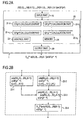
- Fig. 2B is a block diagram for illustrating a configuration of four GF(p d ⁇ m ) calculation parts 22-1 to 22-4 in a finite field calculation part 20.
- the finite field calculation apparatus 1 has an input part 10, the finite field calculation part 20 and an output part 30.
- the finite field calculation part 20 has one or more GF(p m ) calculation parts 21-1 to 21- ⁇ 1 ( ⁇ 1 ⁇ 1) that perform a calculation over the finite field GF(p d ⁇ m ), four or more GF(p m ) calculation parts 22-1 to 22- ⁇ 2 ( ⁇ 2 ⁇ 4) that perform a calculation over the finite field GF(p d ⁇ m ), a control part 23 and a memory 24.
- the finite field calculation part 1 is formed by a well-known computer having a central processing unit (CPU), a random-access memory (RAM), a read-only memory (ROM), an input/output interface and the like with a predetermined program loaded therein. That is, the GF(p m ) calculation parts 21-1 to 21- ⁇ 1 , the GF(p d ⁇ m ) calculation parts 22-1 to 22- ⁇ 2 and the control part 23 are functional parts that are implemented by a predetermined program read in by the CPU, and the memory 24 is a RAM, a cache memory, a register or a hard disk, for example. At least a part of the finite field calculation part 20 may be formed by an integrated circuit.
- FIG. 3 is a diagram for schematically illustrating a process performed by the finite field calculation apparatus 1 according to this embodiment.
- Fig. 4 is a diagram for illustrating characteristics of a calculation performed by a calculation part 22-3.
- each processing performed in the finite field calculation apparatus 1 described below is performed under the control of the control part 23. Every data output from each calculation part is stored in the memory 24. The calculation part reads data from the memory 24 and uses the data for calculation as required.
- N*K elements R(i, k) ⁇ GF(p m ) of the finite field GF(p m ) are first input to the input part 10 and then passed to the finite field calculation part 20.
- the output part 30 outputs the received calculation result.
- the calculation e(R(i, 0), ..., R(i, K-1)) over the finite field GF(p m ) includes, as a part thereof, an extension field calculation over the d-th-order extension field GF(p d ⁇ m ) (d ⁇ 2) of the finite field GF(p m ).
- the extension field calculation is a calculation that maps images on the finite field GF(p m ) that depend on input one or more elements R(i, k) ⁇ ⁇ R(i, 0), ..., R(i, K-1) ⁇ of the finite field GF(p m ) and/or the elements R(i, k) ⁇ ⁇ R(i, 0), ..., R(i, K-1) ⁇ to a polynomial poly (R(i, 0), ..., R(i, K-1)) ⁇ GF(p d ⁇ m ) that expresses elements of the d-th-order extension field GF(p d ⁇ m ). That is, the extension field calculation is mapping from the finite field GF(p m ) to the d-th-order extension field GF(p d ⁇ m ).
- coefficients a h of some terms h ⁇ ⁇ 0, ..., d-1 ⁇ are images on the finite field GF(p m ) that depend on one or more elements R(i, k) of the finite field GF(p m ) and/or the elements R(i, k) of the finite field GF(p m ), and coefficients a r of predetermined terms r ⁇ ⁇ 0, ..., d-1 ⁇ (r ⁇ h) are previously determined to be 0 ⁇ GF(p m ).
- a specific example of such an extension field calculation is a calculation over the sixth-order extension field GF(3 6m) according to the improved ⁇ T pairing calculation algorithm described above. That is, the calculations according to the following formulas (11) and (12) are specific examples of the extension field calculation described above.
- f - y 1 ⁇ u + y 2 ⁇ ⁇ + y 1 ⁇ ⁇ ⁇ GF 3 6 ⁇ m
- g - u 2 + y 1 ⁇ y 2 ⁇ ⁇ - u ⁇ ⁇ - ⁇ 2 ⁇ GF 3 6 ⁇ m
- the maximum value of the number of terms of the polynomial that expresses the elements of the sixth-order extension field GF(p d ⁇ m ) of the finite field GF(p m ) is 6.
- the distortion mapping described below is also an example of the extension field calculation having the characteristics described above. - x 2 + ⁇ ⁇ GF 3 6 ⁇ m y 2 ⁇ ⁇ ⁇ GF 3 6 ⁇ m
- the extension field calculation included in the calculation e(R(i, 0), ..., R(i, K-1)) described above is performed by the GF(p d ⁇ m ) calculation part 22 in the finite field calculation part 20 shown in Fig. 2B .
- images on the finite field GF(p m ) that depend on one or more elements R(i 1 , k) (i 1 ⁇ ⁇ 0, ..., N-1 ⁇ ) of the finite field GF(p m ) and/or the elements R(i 1 , k) of the finite field GF(p m ) are input to a calculation part 22-1 (first calculation part) in the GF(p d ⁇ m ) calculation part 22.
- the "images on the finite field GF(p m ) that depend on one or more elements R(i 1 , k) of the finite field GF(p m )" are the result of calculation performed by any of the GF(p m ) calculation parts 21 in the finite field calculation part 20.
- a specific example of the calculation result is the result of calculation over the finite field GF(3 m ) according to the improved ⁇ T pairing calculation algorithm described above. That is, the following calculation result is a specific example of the "images on the finite field GF(p m ) that depend on one or more elements R(i 1 , k) of the finite field GF(p m )".
- the calculation part 22-1 performs the extension field calculation described above on the images on the finite field GF(p m ) that depend on one or more elements R(i 1 , k) of the finite field GF(p m ) and/or the elements R(i 1 , k) of the finite field GF(p m ) and outputs the resulting polynomial: poly ⁇ R i 1 0 , ... , R ⁇ i 1 , K - 1 ⁇ GF p d ⁇ m
- images on the finite field GF(p m ) that depend on one or more elements R(i 2 , k) (i 2 ⁇ ⁇ 0, ..., N-1 ⁇ (i 2 ⁇ i 1 )) of the finite field GF(p m ) and/or the elements R(i 2 , k) of the finite field GF(p m ) are input to a calculation part 22-2 (second calculation part) in the GF(p d ⁇ m ) calculation part 22.
- the "images on the finite field GF(p m ) that depend on one or more elements R(i 2 , k) of the finite field GF(p m )" are the result of calculation performed by any of the GF(p m ) calculation parts 21 in the finite field calculation part 20.
- the calculation part 22-2 performs the extension field calculation described above on these images or elements and outputs the resulting polynomial: poly ⁇ R i 2 0 , ... , R ⁇ i 2 , K - 1 ⁇ GF p d ⁇ m
- the polynomials poly(R(i 1 , 0), ..., R(i 1 , K-1)) and poly(R(i 2 , 0), ..., R(i 2 , K-1)) described above are input to the calculation part 22-3 (third calculation part) in the GF(p d ⁇ m ) calculation part 22.
- the calculation part 22-3 determines their product poly ⁇ R i 1 0 , ... , R ⁇ i 1 , K - 1 ⁇ poly ⁇ R i 2 0 , ... , R ⁇ i 2 , K - 1 ⁇ GF p d ⁇ m and outputs the product poly(R(i 1 , 0), ..., R(i 1 , K-1)) ⁇ poly(R(i 2 , 0), ..., R(i 2 , K-1)) ⁇ GF(p d ⁇ m ) .
- the calculation part 22-3 in this embodiment determines the product poly(R(i 1 , 0), ..., R(i 1 , K-1)) ⁇ poly(R(i 2 , 0), ..., R(i 2 , K-1)) without performing any calculation that involves as operands the terms of the polynomial poly(R(i 1 , 0), ..., R(i 1 , K-1)) that are previously determined to be 0 ⁇ GF(p m ) and/or the terms of the polynomial poly(R(i 2 , 0), ..., R(i 2 , K-1)) that are previously determined to be 0 ⁇ GF(p m ).
- the calculation part 22-3 determines the product thereof over the sixth-order extension field GF(p 6m ).
- the coefficients of the indeterminate elements p* ⁇ and p 2 * ⁇ of each polynomial are previously determined to be 0, and thus, no calculation that involves the coefficients of the indeterminate elements p* ⁇ and p2* ⁇ as operands is not performed.
- the calculation amount is reduced by performing a multiplication of polynomials the coefficients of some of the terms of which are previously determined to be 0.
- the control part 23 makes the calculation parts 22-1 to 22-3 perform a loop process (horizontal loop) in which the series of processing stages are performed L/2 times while changing the values i 1 and i 2 in such a manner that each element of a subset including L (which represents an even number) different elements of the set ⁇ 0,..., N-1 ⁇ is used one time as i 1 or i 2 .
- control part 23 selects each element of a subset including L (which represents an even number) different elements of the set ⁇ 0,..., N-1 ⁇ one time as i 1 and i 2 , and makes the calculation parts 22-1 to 22-3 perform the series of processing stages thereof one time for each pair of selected i 1 and i 2 , thereby performing a loop process including the series of processing stages for the L/2 pairs (i 1 , i 2 ).
- the calculation part 22-4 may successively stores the products poly(R(i 1 , 0), ..., R(i 1 , K-1)) ⁇ poly(R(i 2 , 0), ..., R(i 2 , K-1)) output from the calculation part 22-3 as results of the series of processing stages in the memory 24 and calculate the multiplication value thereof after the products are completely calculated.
- the calculation part 22-4 preferably determines the multiplication value each time one series of processing stages is performed by multiplying the previous multiplication value (the initial value is 1, the multiplicative identity element) by the product poly(R(i 1 , 0), ..., R(i 1 , K-1)) ⁇ poly(R(i 2 , 0), ..., R(i 2 , K-1)) output from the calculation part 22-3.
- the multiplication value of the products poly(R(i 1 , 0), ..., R(i 1 , K-1)) ⁇ poly(R(i 2 , 0), ..., R(i 2 , K-1)) which have been obtained is preferably updated.
- This embodiment is an example in which the present invention is applied to the part of calculation of g of the improved ⁇ T pairing calculation algorithm.
- Figs. 5 and 6 are block diagrams for illustrating a basic configuration of a finite field calculation part 120 according to the first embodiment.
- a finite field calculation apparatus is the finite field calculation apparatus shown in Fig. 2A with the finite field calculation part 20 replaced with the finite field calculation part 120 shown in Figs. 5 and 6 .
- the following description will be focused only on the configuration of the finite field calculation part 120.
- the finite field calculation part 120 has GF(3 m ) calculation parts 121-1 to 121-4 that perform a calculation over the finite field GF(3 m ), GF(3 6m) calculation parts 122-1 to 122-9 that perform a calculation over the sixth-order extension field GF(3 6m) of the finite field GF(3 m ), a control part 123, a memory 124 and a GF(3) calculation part 125 that performs a calculation over a finite field GF(3).
- the finite field calculation part 120 is a special device that comprises a well-known or dedicated computer having a CPU, a RAM and a ROM, for example, and a special program. That is, the GF(3 m ) calculation parts 121-1 to 121-4, the GF(3 6m) calculation parts 122-1 to 122-9, the GF(3) calculation part 125 and the control part 123 are functional parts that are implemented by a predetermined program read in by the CPU, and the memory 124 is a RAM, a cache memory, a register or a hard disk, for example. At least a part of the finite field calculation part 120 may be formed by an integrated circuit.
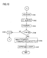
- Figs. 7 to 10 are diagrams for illustrating a process according to the first embodiment. In the following, the process according to the first embodiment will be described with reference to these drawings.
- affine coordinate points X 1 [i], Y 1 [i], X 2 [i] and Y 2 [i] ⁇ GF(p m ) (i ⁇ ⁇ 0, ..., N-1 ⁇ ) of two points P(X 1 [i], Y 1 [i]) and Q(X 2 [i], Y 2 [i]) on the supersingular elliptic curve E b , which are input values for each pairing calculation e(P(X 1 [i], Y 1 [i]), Q(X 2 [i], Y 2 [i])) forming the multi-pairing calculation ⁇ i 0 N-1 e(P(X 1 [i], Y 1 [i]), Q(X 2 [i], Y 2 [i])), are input to the input part 10 ( Fig.
- the affine coordinate points X 1 [i], Y 1 [i], X 2 [ i ] and Y 2 [ i ] ⁇ GF(3 m ) stored in the memory 124 are denoted as x 1 [i], y 1 [i], x 2 [i] and y 2 [i] ⁇ GF(3 m ), respectively (step S101).
- the GF(3 6m ) calculation part 122-3 determines the product g[0] ⁇ g[1] ⁇ GF(3 6m ) without performing any calculation that involves as operands the terms, being previously determined to be 0 ⁇ GF(p m ), of the calculation result g[0] and/or the calculation result g[1].
- the GF(3 6m ) calculation part 122-3 (third calculation part) reads the calculation results g[i] ⁇ GF(3 6m ) and g[i+1] ⁇ GF(3 6m ) from the memory 124, performs the following calculation g i ⁇ g ⁇ i + 1 ⁇ GF 3 6 ⁇ m and stores the calculation result g[i] ⁇ g[i+1] ⁇ GF(3 6m ) in the memory 124 (step S131).
- the GF(3 6m ) calculation part 122-3 determines the product g[i] ⁇ g[i+1] ⁇ GF(3 6m ) without performing any calculation that involves as operands the terms, being previously determined to be 0 ⁇ GF(p m ), of the calculation result g[i] and/or the calculation result g[i+1].
- the GF(3 6m ) calculation part 122-3 determines the multiplication value of the products g[i] ⁇ g[i+1] output from the GF(3 6m ) calculation part 122-3 (third calculation part). As described above, this allows saving of the capacity of the memory 124.
- steps S141 to S143 are performed each time the "loop process (steps S115 to S140)", in which the "series of processing stages” performed by the GF(3 6m ) calculation part 122-1 (first calculation part), the GF(3 6m ) calculation part 122-2 (second calculation part) and the GF(3 6m ) calculation part 122-3 (third calculation part) is performed N/2 times, is performed.
- the calculation result output ⁇ GF(3 6m ) is output from the output part 30 ( Fig. 2A ).
- g i - u i 2 + y 1 i ⁇ y 2 i ⁇ ⁇ - u i ⁇ ⁇ - ⁇ 2 ⁇ GF 3 6 ⁇ m
- g ⁇ i + 1 - u ⁇ i + 1 2 + y 1 ⁇ i + 1 ⁇ y 2 ⁇ i + 1 ⁇ ⁇ - u ⁇ i + 1 ⁇ ⁇ - ⁇ 2 ⁇ GF 3 6 ⁇ m
- the product thereof is determined as follows.
- the following calculation is performed using the products (steps S119 to S121, steps S129 to S132).
- the coefficients of the terms of the indeterminate elements ⁇ ⁇ GF(p 6m ) and ⁇ 2 ⁇ ⁇ GF(p 6m ) of the polynomials (60) and (61) that express the sixth-order extension field GF(3 6m ) are previously determined to be 0. Since the product of such polynomials is calculated in advance, the terms whose coefficients are previously determined to be 0 do not have to be calculated, and therefore, the number of multiplications can be reduced.
- « ⁇ M» represents ⁇ multiplications
- « ⁇ C» represents ⁇ cubic calculations
- g[0] and g[1] are determined according to the formulas (64) and (65), and then the product thereof is determined according to the formula (66).
- g[i] and g[i+1] are determined according to the formulas (67) and (68), and then the product thereof is determined according to the formula (70).
- the number of multiplications can be substantially reduced by performing the calculations in the order according to this embodiment.
- the prior-art literatures 1 and 2 disclose no methods for efficient calculation of the product of a plurality of pairings. In the following, it will be shown that the calculation amount cannot be reduced more substantially than this embodiment even if the improved ⁇ T pairing calculation algorithm disclosed in the prior-art literature 1 is simply extend to the multi-pairing calculation.
- the prior-art literature 2 discloses no method for efficient calculation of the product of a plurality of pairings.
- the prior-art literature 2 discloses an algorithm based on the loop unrolling. In the following, it will be shown that the calculation amount cannot be reduced more substantially than this embodiment even if the concept of the algorithm based on the loop unrolling disclosed in the prior-art literature 2 is extend to the multi-pairing calculation.
- the polynomials - ⁇ u[i] ⁇ 2 +y 1 [i] ⁇ y 2 [i] ⁇ -u[i] ⁇ - ⁇ 2 are separately determined for different pairings for different values of i, respectively, and the product thereof is determined.
- cubic calculations in the formulas (76) and (80) are needed.
- the first embodiment concerns a case where N is an even number equal to or greater than 4.
- a modification of the first embodiment described below concerns a case where N is an odd number equal to or greater than 5.
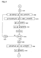
- control part 123 sets i+2 as a new i and stores the setting in the memory 124 (step S160).
- the first embodiment is an example in which the present invention is applied to the part of calculation of g of the improved ⁇ T pairing calculation algorithm.
- the present invention is applied to the parts of calculation of both f and g of the improved ⁇ T pairing calculation algorithm. This allows further reduction of the calculation amount.
- g i - u i 2 + y 1 i ⁇ y 2 i ⁇ ⁇ - u i ⁇ ⁇ - ⁇ 2 ⁇ GF 3 6 ⁇ m
- the affine coordinate points X 1 [i], Y 1 [i], X 2 [i] and Y 2 [i] input to the input part or the images thereof are represented by x 1 [i],
- Figs. 12 and 13 are block diagrams for illustrating a basic configuration of a finite field calculation part 220 according to the second embodiment.
- a finite field calculation apparatus is the finite field calculation apparatus shown in Fig. 2A with the finite field calculation part 20 replaced with the finite field calculation part 220 shown in Figs. 12 and 13 .
- the following description will be focused only on the configuration of the finite field calculation part 220.
- the finite field calculation part 220 has GF(3 m ) calculation parts 121-1 to 121-4 that perform a calculation over the finite field GF(3 m ), GF(3 6m ) calculation parts 122-1 to 122-5 and 122-9 that perform a calculation over the sixth-order extension field GF(3 6m ) of the finite field GF(3 m ), GF(3 6m ) calculation parts 222-1 to 222-5, a control part 123, a memory 124 and a GF(3) calculation part 125 that performs a calculation over the finite field GF(3).
- the finite field calculation part 220 is a special device that comprises a well-known or dedicated computer having a CPU, a RAM and a ROM, for example, and a special program.
- the GF(3 6m ) calculation parts 222-1 to 222-5 are functional parts that are implemented by a predetermined program read in by the CPU. At least a part of the finite field calculation part 220 may be formed by an integrated circuit.
- Figs. 14 to 15 are diagrams for illustrating a process according to the second embodiment. In the following, the process according to the second embodiment will be described with reference to these drawings.
- the GF(3 6m ) calculation part 222-3 determines a product f[0] ⁇ f[1] ⁇ GF(3 6m ) without performing any calculation that involves as operands the terms, being previously determined to be 0 ⁇ GF(p m ), of the calculation result f[0] and/or the calculation result f[1].
- the GF(3 6m ) calculation part 222-3 reads the calculation results f[i] ⁇ GF(3 6m ) and f[i+1] ⁇ GF(3 6m ) from the memory 124, performs the following calculation f i ⁇ f ⁇ i + 1 ⁇ GF 3 6 ⁇ m and stores the calculation result f[i] ⁇ f[i+1] ⁇ GF(3 6m ) in the memory 124 (step S212).
- the GF(3 6m ) calculation part 222-3 determines a product f[i] ⁇ f[i+1] ⁇ GF(3 6m ) without performing any calculation that involves as operands the terms, being previously determined to be 0 ⁇ GF(p m ), of the calculation result f[i] and/or the calculation result f[i+1].
- f i - y 1 i ⁇ x 1 i + x 2 i + b + y 2 i ⁇ ⁇ + y 1 i ⁇ ⁇ ⁇ GF 3 6 ⁇ m
- f ⁇ i + 1 - y 1 ⁇ i + 1 ⁇ x 1 ⁇ i + 1 + x 2 ⁇ i + 1 + b + y 2 ⁇ i + 1 ⁇ ⁇ + y 1 ⁇ i + 1 ⁇ ⁇ ⁇ GF 3 6 ⁇ m
- the product thereof is determined as follows.
- the coefficients of the terms of the indeterminate elements ⁇ 2 ⁇ GF(p 6m ), ⁇ ⁇ GF(p 6m ) and ⁇ 2 ⁇ ⁇ GF(p 6m ) of the polynomials (95) and (96) that express the sixth-order extension field GF(3 6m ) are previously determined to be 0. Since the product of such polynomials is calculated in advance, the terms whose coefficients are previously determined to be 0 do not have to be calculated, and therefore, the number of multiplications can be reduced.
- the second embodiment concerns a case where N is an even number equal to or greater than 4.
- a modification of the second embodiment described below concerns a case where N is an odd number equal to or greater than 5.
- control part 123 sets i+2 as a new i and stores the setting in the memory 124 (step S255).
- the first embodiment is an example in which the present invention is applied to the part of calculation of g of the improved ⁇ T pairing calculation algorithm.
- the present invention is applied to only the part of calculation of f of the improved ⁇ T pairing calculation algorithm.
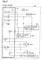
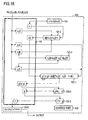
- Figs. 17 and 18 are block diagrams for illustrating a basic configuration of a finite field calculation part 320 according to the third embodiment.
- a finite field calculation apparatus according to the third embodiment is the finite field calculation apparatus shown in Fig. 2A with the finite field calculation part 20 replaced with the finite field calculation part 320 shown in Figs. 17 and 18 .
- the following description will be focused only on the configuration of the finite field calculation part 320.
- the finite field calculation part 320 has GF(3 m ) calculation parts 121-1 to 121-4 that perform a calculation over the finite field GF(3 m ), GF(3 6m ) calculation parts 122-1 to 122-5 and 122-9 that perform a calculation over the sixth-order extension field GF(3 6m ) of the finite field GF(3 m ), GF(3 6m ) calculation parts 222-1 to 222-5, GF(3 6m ) calculation parts 322-1 and 322-2, a control part 123, a memory 124 and a GF(3) calculation part 125 that performs a calculation over the finite field GF(3).
- the finite field calculation part 320 is a special device that comprises a well-known or dedicated computer having a CPU, a RAM and a ROM, for example, and a special program.
- the GF(3 6m ) calculation parts 322-1 and 322-2 are functional parts that are implemented by a predetermined program read in by the CPU. At least a part of the finite field calculation part 320 may be formed by an integrated circuit.
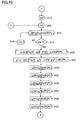
- Figs. 19 to 20 are diagrams for illustrating a process according to the third embodiment. In the following, the process according to the third embodiment will be described with reference to these drawings.
- a loop process can be performed in which the series of processing stages performed by the first calculation part, the second calculation part and the third calculation part is performed L/2 times while changing i 1 and i 2 in such a manner that each element of a subset including L (which represents an even number) different elements of the set ⁇ 0, ..., N-1 ⁇ is used one time as i 1 or i 2 , and the series of processing stages performed by the sixth calculation part, the seventh calculation part and the eighth calculation part can be performed W/2 times while changing i 3 and i 4 in such a manner that each element of a subset comprising W (which represents a positive even number) different elements of the set ⁇ 0, ..., N-1 ⁇ is used one time as i 3 or i 4 .
- each element of a subset including L (which represents an even number) different elements of the set ⁇ 0, ..., N-1 ⁇ is selected one time as i 1 or i 2 , and first processing stages, each of which includes processing stages performed by the first calculation part, the second calculation part and the third calculation part are performed one time for each pair of selected i 1 and i 2 , thereby performing the first processing stages for the L/2 pairs (i 1 , i 2 ), respectively.
- each element of a subset comprising W (which represents a positive even number) different elements of the set ⁇ 0, ..., N-1 ⁇ is selected one time as i 3 or i 4 , and second processing stages, each of which includes processing stages performed by the sixth calculation part, the seventh calculation part and the eighth calculation part one time for each pair of selected i 3 and i 4 , thereby performing the second processing stages for the W/2 pairs (i 3 , i 4 ), respectively.
- other positive even numbers smaller than N may be L and/or W.
- the processing for i to which the method according to the present invention is not applied can be performed by repeating the cumulative calculation in steps S161 and S162 shown in Fig. 11 or steps S256 and S257 shown in Fig. 16 .
- L may not be equal to W.
- N may assume 2 or 3. In that case, the processing stages in steps S108 to S111 and S113 in Fig.
- the parameters such as b, are previously set.
- the parameters may be input to the apparatus.
- the product poly(R(i 1 , 0), ..., R(i 1 , K-1)) ⁇ poly(R(i 2 , 0), ..., R(i 2 , K-1)) is determined without performing any calculation that involves as operands the terms, being previously determined to be 0 ⁇ GF(p m ), of the polynomial poly(R(i 1 , 0), ..., R(i 1 , K-1)) and/or the polynomial poly(R(i 2 , 0), ..., R(i 2 , K-1)).
- a calculation that involves as operands some of these terms that are previously determined to be 0 ⁇ GF(p m ) may be performed.
- the present invention is applied to the improved ⁇ T pairing calculation algorithm of characteristic 3.
- the present invention may be applied to other pairing calculations in characteristic 3, pairing calculations in characteristic 2, or pairing calculations in other characteristics.
- the program that describes the specific processings can be recorded in a computer-readable recording medium.
- the computer-readable recording medium may be any type of recording medium, such as a magnetic recording device, an optical disk, a magneto-optical recording medium and a semiconductor memory.
- the program may be distributed by selling, transferring or lending a portable recording medium, such as a DVD and a CD-ROM, in which the program is recorded, for example.
- the program may be distributed by storing the program in a storage device in a server computer and transferring the program from the server computer to other computers via a network.
- the computer that executes the program first temporarily stores, in a storage device thereof, the program recorded in a portable recording medium or transferred from a server computer, for example. Then, when performing the processings, the computer reads the program from the recording medium and performs the processings according to the read program.
- the computer may read the program directly from the portable recording medium and perform the processings according to the program.
- the computer may perform the processings according to the program each time the computer receives the program transferred from the server computer.
- the processings described above may be performed on an application service provider (ASP) basis, in which the server computer does not transmit the program to the computer, and the processings are implemented only through execution instruction and result acquisition.
- the programs according to the embodiments of the present invention include a quasi-program, which is information processed by a computer (data or the like that is not a direct instruction to a computer but has a property that defines the processings performed by the computer).
- Industrial applications of the present invention include cryptographic applications that use a multi-pairing calculation, such as the inner product predicate encryption.
Landscapes
- Engineering & Computer Science (AREA)
- General Physics & Mathematics (AREA)
- Theoretical Computer Science (AREA)
- Physics & Mathematics (AREA)
- Mathematical Analysis (AREA)
- Mathematical Optimization (AREA)
- Pure & Applied Mathematics (AREA)
- Computing Systems (AREA)
- Mathematical Physics (AREA)
- Algebra (AREA)
- Computer Security & Cryptography (AREA)
- Computer Networks & Wireless Communication (AREA)
- Signal Processing (AREA)
- Computational Mathematics (AREA)
- General Engineering & Computer Science (AREA)
- Complex Calculations (AREA)
Abstract
Description
- The present invention relates to a cryptographic technique. In particular, it relates to a technique of calculation over a finite field.
- In recent years, with the practical use of cryptographic schemes based on pairing, studies to improve the pairing efficiency have become more active. The pairing is a two-input one-output bilinear function. The present cryptography uses a pairing that accepts as inputs two points P(x1, y1) and Q(x2, y2) on an elliptic curve defined on a finite field GF(pm) (x1, y1, x2, y2 ∈ GF(pm), p represents a prime number, and m represents an integer equal to or greater than 1) and returns an element ηT(P,Q) of an extension field GF(pd·m) of the finite field GF(pm) (ηT(P, Q) ∈ GF(3d·m)):

- The first proposed algorithm for pairing calculation in polynomial time is the Miller algorithm for Tate pairing. Following the Miller algorithm, the ηT pairing algorithm, which is reduced by half in number of recursions compared with the Miller algorithm, and then the improved ηT pairing algorithm, which is further improved in calculation speed by omitting the cube root calculation involved with the ηT pairing algorithm, were proposed (see Non-patent
literature 1, for example). In the following, the improved ηT pairing algorithm will be summarized. -
- Eb: Eb represents a supersingular elliptic curve that is defined on a finite field GF(3m) and expressed as Y2 = X3-X+b (b ∈ {-1,1}).
- σ: σ represents an indeterminate element that is a root of an irreducible polynomial σ2+1 = 0 over the finite field GF(3m).
- ρ: ρ represents an indeterminate element that is a root of a polynomial ρ3-ρ-b = 0 over the finite field GF(3m).
- [Input] P(x1, y1), Q(x2, y2)(x1, y1, x2, y2 ∈ GF(3m))
- [Output] ηT(P, Q) ∈ GF(36m)
- [Calculation Process]
- Step 1: y1 = -y1 ∈ GF(3m) (only if b = 1)
- Step 2: u = x1+x2+b ∈ GF(3m)
- Step 3: c = b
- Step 4: f = -y1·u+y2·σ+y1·ρ ∈ GF(36m)
- Step 5: repeat Steps 5-1 to 5-8 while increasing j from 0 to (m-1)/2 in increments of 1
-
- Step 5-1: u = x1+x2+c ∈ GF(3m)
- Step 5-2: g = -u2+y1·y2·σ-u·ρ-ρ2 ∈ GF(36m)
- Step 5-3: f = f·g ∈ GF(36m)
- Step 5-4: f = f3 ∈ GF(36m)
- Step 5-5: y1 = -y1 ∈ GF(3m)
- Step 5-6: x2 = x2 9 ∈ GF(3m)
- Step 5-7: y2 = y2 9 ∈ GF(3m)
- Step 5-8: c = (c-b)
mod 3 ∈ GF(3) - Step 6: output ffinalpow ∈ GF(36m)[finalpow = (33m-1)(3m+1)(3m - 3(m+1)/2+1)]
-
Non-patent literature 2 discloses an algorithm that is obtained by applying the loop unrolling technique, which is a kind of loop transformation, to the ηT pairing calculation. The loop unrolling technique is to improve the execution speed by decreasing the number of determination steps for loop termination, which occur in every repeated loop. According to the method disclosed inNon-patent literature 2, a processing that involves two loops according to the basic algorithm is performed in one loop to reduce the number of loop repetitions by half, thereby reducing the number of determination steps for loop termination by half. - Non-patent literature 1: Beuchat, J.-L.; Shirase, M.; Takagi, T.; Okamoto, "An Algorithm for the ηT Pairing Calculation in Characteristic Three and its Hardware Implementation", Proceedings of the 18th IEEE Symposium on Computer Arithmetic, Institute of Electrical and Electronics Engineers, 25-27 June 2007, pp. 97-104
Non-patent literature 2: Beuchat, J.-L.; Brisebarre, N.; Detrey, J.; Okamoto, E.; Shirase, M.; Takagi, T., "Algorithms and Arithmetic Operators for Computing the ηT Pairing in Characteristic Three", IEEE transactions on computers, Institute of Electrical and Electronics Engineers, Nov. 2008, Volume 57, Issue 11, pp. 1454-1468 - The prior-
art literatures - Suppose that a pairing that accepts as inputs two points P(X1[i], Y1[i]) and Q(X2[i], Y2[i]) (X1[i], Y1[i], X2[i], Y2[i] ∈ GF(pm)) on an elliptic curve defined on a finite field GF(pm) and returns an element ηT(P[i], Q[i]) of an extension field GF(pd·m) of the finite field GF(pm) (ηT(P[i], Q[i]) ∈ GF(3d·m)) is expressed as follows:

art literatures 
- According to the conventional methods disclosed in the prior-
art literatures - The same holds true for calculations other than pairing. For example, supposing that a calculation of K elements R(1, 0), ..., R(1, K-1) ∈ GF(pm) (i ∈ {0, ..., N-1}) over a finite field is expressed as


where R(i, k) ∈ GF(pm), N ≥ 2, K ≥ 1, i ∈ {0,...,N-1},k∈ {0,...,K-1},p represents a prime number, and m represents an integer equal to or greater than 1. -
Fig. 1 is a conceptual diagram for illustrating a conventional method for calculating the formula (5).Fig. 1 shows an example in which N =6,and i=0,...,5. - As shown in
Fig. 1 , in calculation of the formula (5) according to the conventional method, a plurality of calculations (a set of calculations in a dotted-line square) including calculations for the finite field GF(pm) and calculations for the extension field GF(pm) is performed for each value of i. Then, the results e(R(i, 0), ..., R(i, K-1)) of the calculations for the different values of i are multiplied on the extension field GF(pm) to obtain the result of the calculation of the formula (5). - However, the calculation of the formula (5) can be improved in efficiency by finding an ingenious way of cooperation of the calculations of the formula (4) for the different values of i.
- The present invention has been devised in view of such circumstances, and an object of the present invention is to provide a technique of efficiently calculating Πi=0 N-1e(R(i, 0), ..., R(i, K-1)) where e(R(i, 0), ..., R(i, K-1)) represents a calculation of K elements R(i, 0), ..., R(i, K-1) ∈ GF(pm) of the finite field GF(pm) over a finite field.
- According to the present invention, N*K elements R(i, k) ∈ GF(pm) of a finite field GF(pm) are input (N ≥ 2, K ≥ 1, i ∈ {0, ..., N-1}, k ∈ {0, ..., K-1}, p represents a prime number, and m represents an integer equal to or greater than 1), a finite field calculation part performs a calculation Πi=0 N-1e(R(i,0), ..., R(i, K-1)) where e(R(i, 0), ..., R(i, K-1)) represents a calculation of K elements R(i, 0), ..., R(i, K-1) ∈ GF(pm) of the finite field GF(pm) over a finite field, and the result of the calculation is output.
- The calculation e(R(i, 0), ... ,R(i, K-1)) over the finite field includes an extension field calculation over a d-th-order extension field GF(pd·m) (d ≥ 2) of the finite field GF(pm). The extension field calculation is a calculation that maps images over the finite field GF(pm) that depend on one or more input elements R(i, k) ∈ {R(i, 0), ..., R(i, K-1)} of the finite field GF(pm) and/or the elements R(i, k) ∈ {R(i, 0), ..., R(i, K-1)} of the finite field GF(pm) to a polynomial poly(R(i, 0), ..., R(i, K-1)) ∈ GF(pd·m) that expresses an element of the d-th-order extension field GF(pd·m). The polynomial poly(R(i, 0), ..., R(i, K-1)) ∈ GF(pd·m) is a polynomial having d terms, the coefficients ah of some of the terms h ∈ {0, ..., d-1} of which are the images over the finite field GF(pm) that depend on one or more input elements R(i, k) of the finite field GF(pm) and/or the elements R(i, k) of the finite field GF(pm), and the coefficients ar of predetermined some of the terms r ∈ {0, ..., d-1} (r≠ h) of which are previously determined to be 0 ∈ GF(pm). That is, at least some of the coefficients in the polynomial poly(R(i, 0), ..., R(i, K-1)) ∈ GF(pd·m) are 0 at any time.
- A first calculation part of the finite field calculation part receives, for any i1 ∈ {0, ..., N-1}, images over the finite field GF(pm) that depend on one or more elements R(i1, k) of the finite field GF(pm) and/or the elements R(i1, k) of the finite field GF(pm), performs the extension field calculation therefor, and outputs the resulting polynomial poly(R(i1, 0), ..., R(i1, K-1)) ∈ GF(pd·m). A second calculation part of the finite field calculation part receives, for any i2 ∈ {0, ..., N-1} (i2 ≠ i1), images over the finite field GF(pm) that depend on one or more elements R(i2, k) of the finite field GF(pm) and/or the elements R(i2, k) of the finite field GF(pm), performs the extension field calculation therefor, and outputs the resulting polynomial poly(R(i2, 0), ..., R(i2, K-1)) ∈ GF(pd·m). A third calculation part of the finite field calculation part receives the polynomial poly(R(i1, 0), ..., R(i1, K-1)) and the polynomial poly(R(i2, 0), ..., R(i2, K-1)), calculates the product thereof poly(R(i1, 0), ..., R(i1, K-1))·poly(R(i2, 0), ..., R(i2, K-1)) ∈ GF(pd·m) , and outputs the product poly(R(i1, 0), ..., R(i1, K-1))·poly(R(i2, 0), ..., R(i2, K-1)).
- Each element of a subset including L (which represents an even number) different elements of the set {0,..., N-1} is selected one time as i1 or i2, and the first calculation part, the second calculation part and the third calculation part perform respective processing stages one time for each pair of selected i1 and i2, thereby performing a loop process including the processing stages for the L/2 pairs of i1 and i2. Using the products poly(R(i1, 0), ..., R(i1, K-1))·poly(R(i2, 0), ..., R(i2, K-1)) obtained by the processings, Πi=0 N-1poly(R(i, 0), ..., R(i, K-1)) ∈ GF(pd·m) is calculated.
- As described above, at least some of the coefficients in the polynomial poly(R(i, 0), ..., R(i, K-1)) ∈ GF(pd·m) and the polynomial poly(R(i2, 0), ..., R(i2, K-1)) ∈ GF(pd·m) are 0 at any time. Since the product of such polynomials is calculated in advance, calculations applying the coefficients that are 0 are unnecessary, and therefore, the amount of multiplication is reduced.
- According to the present invention, the calculation Πi=0 N-1e(R(i,0), ..., R(i, K-1)) where e(R(i, 0), ..., R(i, K-1)) represents a calculation of K elements R(i, 0), ..., R(i, K-1) ∈ GF(pm) of the finite field GF(pm) over a finite field can be efficiently performed.
-
-
Fig. 1 is a conceptual diagram for illustrating a conventional method for calculating the formula (5); -
Fig. 2A is a block diagram for illustrating a basic configuration of a finite field calculation apparatus according to an embodiment; -
Fig. 2B is a block diagram for illustrating a configuration of four GF(pd·m) calculation parts in the finite field calculation part; -
Fig. 3 is a diagram for schematically illustrating a process performed by the finite field calculation apparatus according to an embodiment; -
Fig. 4 is a diagram for illustrating characteristics of a calculation performed by a calculation part; -
Fig. 5 is a block diagram for illustrating a basic configuration of a finite field calculation part according to a first embodiment; -
Fig. 6 is a block diagram for illustrating a basic configuration of the finite field calculation part according to the first embodiment; -
Fig. 7 is a diagram for illustrating a process according to the first embodiment; -
Fig. 8 is a diagram for illustrating the process according to the first embodiment; -
Fig. 9 is a diagram for illustrating the process according to the first embodiment; -
Fig. 10 is a diagram for illustrating the process according to the first embodiment; -
Fig. 11 is a diagram for illustrating a process in a case where N is an odd number equal to or greater than 5; -
Fig. 12 is a block diagram for illustrating a basic configuration of a finite field calculation part according to a second embodiment; -
Fig. 13 is a block diagram for illustrating a basic configuration of the finite field calculation part according to the second embodiment; -
Fig. 14 is a diagram for illustrating a process according to the second embodiment; -
Fig. 15 is a diagram for illustrating the process according to the second embodiment; -
Fig. 16 is a diagram for illustrating a process in a case where N is an odd number equal to or greater than 5; -
Fig. 17 is a block diagram for illustrating a basic configuration of a finite field calculation part according to a third embodiment; -
Fig. 18 is a block diagram for illustrating a basic configuration of the finite field calculation part according to the third embodiment; -
Fig. 19 is a diagram for illustrating a process according to the third embodiment; and -
Fig. 20 is a diagram for illustrating the process according to the third embodiment. - In the following, embodiments of the present invention will be described with reference to the drawings.
- First, definitions of the terms and symbols used herein will be provided.
- p: p represents a positive prime number. Specific examples of "p" include 2 and 3.
- m: m represents an integer equal to or greater than 1. Specific examples of "m" include odd numbers and prime numbers equal to or greater than 3. In cryptography, values of 97, 167, 193, 239, 353 and 509 are commonly used as m, for example.
- d: d represents an integer equal to or greater than 2.
- L: L represents a positive even number.
- N: N represents an integer equal to or greater than 2.
- K: K represents an integer equal to or greater than 1.
- i: i represents an element included in a set {0, ..., N-1}.
- k: k represents an element included in a set {0, ..., K-1}.
- GF(p): GF(p) represents a finite field whose order (number of elements) is p. The order p is a prime number, and therefore, the finite field GF(p) is a prime field. For example, the finite field GF(p) is formed by a remainder of division modulo p:

The calculation over the finite field GF(p) can be implemented simply by a remainder calculation modulo p, for example. A multiplication β*γ ∈ GF(p) over the finite field GF(p) can be implemented by (β*γ) mod p, and an addition β+γ ∈ GF(p) over the finite field GF(p) can be implemented by (β+γ) mod p. - GF(pm): For m ≥ 2, GF(pm) represents an extension field whose order is pm, which is an m-th-order extension of the finite field GF(p). For m = 1, GF(pm) represents a prime field that satisfies a relationship of GF(pm)= GF(p).
- The extension field GF(pm), which is the m-th-order extension of the finite field GF(p), can be formed by a single-variable or multi-variable m-term polynomial whose indeterminate elements are roots of an irreducible polynomial over the finite field GF(p) and whose coefficients are elements of the finite field GF(p). For example, in the case where the extension field GF(pm) is formed by a single-variable polynomial, the extension field GF(pm) is formed by the following polynomial:

whose indeterminate elements ω ∈ GF(pm) are roots of an m-th-order irreducible polynomial ipoly(ω) = 0 over the finite field GF(p) and whose coefficients κ0, ..., κm-1 ∈ GF(p) are elements of the finite field GF(p). A specific example of mapping of elements of the finite field GF(p) to elements of the extension field GF(pm) is distortion mapping. The term "coefficient" used herein includes a coefficient of a constant term. - An addition over the extension field GF(pm) can be implemented as an addition of polynomials expressing the extension field GF(pm). However, an addition of coefficients in the addition of the polynomials is an addition over the finite field GF(p). For example, the result of an addition of κ0+κ1·ω+...+κm-1·ωm-1 ∈ GF(pm) and υ0+υ1·ω+...+υm-1·ωm-1 ∈ GF(pm) (υ0, ..., υm-1 ∈ GF(p)) is {(κ0+υ0)+(κ1+υ1)·ω+...+(κm-1+υm-1)·ωm-1} ∈ GF(pm). Note that (κ0+υ0) ∈ GF(p) and (κ1+υ1) ∈ GF(p), ... and (κm-1+υm-1) ∈ GF(p).
- A multiplication over the extension field GF(pm) can be implemented by taking a remainder of the product of polynomials expressing the extension field GF(pm) modulo an irreducible polynomial whose root is an indeterminate element of the polynomials. For example, a multiplication of κ0+κ1·ω+...+κm-1·ωm-1 ∈ GF(pm) and υ0+υ1·ω+...+υm-1·ωm-1 ∈ GF(pm) can be implemented by taking a remainder of (κ0+κ1·ω+...+κm-1·ωm-1) ·(υ0+υ1·ω+...+υm-1·ωm-1)modulo an irreducible polynomial ipoly(ω). Specifically, the product over the extension field GF(pm) is an m-th or lower order polynomial obtained by substituting the irreducible polynomial ipoly(ω) = 0 to (κ0+κ1·ω+...+κm-1·ωm-1)·(υ0+υ1·ω+...+υm-1·ωm-1).
- GF(pd·m): GF(pd·m) represents a d-th-order extension field of the finite field GF(pm). The d-th-order extension field GF(pd·m) of the finite field GF(pm) can be formed by a single-variable or multi-variable d-term polynomial whose indeterminate elements are roots of an irreducible polynomial over the finite field GF(pm) and whose coefficients are elements of the finite field GF(pm). Although an example in which an extension field is formed by a single-variable polynomial has been described above, an example in which a sixth-order extension field is formed by a two-variable polynomial will be described here.
- Supposing that σ ∈ GF(p6m) for roots σ of an irreducible polynomial ipolyl(ω) over the finite field GF(pm), and p ∈ GF(p6m) for roots of an irreducible polynomial ipoly2(p) over the finite field GF(pm), elements of the finite field GF(p6m) are expressed by the following polynomial, whose coefficients a5, ..., a0 ∈ GF(pm) are elements of the finite field GF(pm).

- An addition over the d-th-order extension field GF(pd·m) can be implemented as an addition of polynomials expressing the d-th-order extension field GF(pd·m). However, an addition of coefficients in the addition of the polynomials is an addition over the finite field GF(pm). For example, the result of an addition of a0+a1·ρ+a2·ρ2+a3·σ+a4·ρ·σ+a5·ρ2·σ ∈ GF(p6m) and υ0+a1·ρ+υ2·ρ2+υ3·σ+υ4·ρ·σ+υ5·ρ2·σ ∈ GF(p6m) (υ5, ..., υ0 ∈ GF(pm)) is expressed as follows:

where (a0+υ0) ∈ GF(pm), and (a1+υ1) ∈ GF(pm), ..., and (a5+υ5) ∈ GF(pm). - A multiplication over the d-th-order extension field GF(pd·m) can be implemented by taking a remainder of the product of polynomials expressing the d-th-order extension field GF(pd·m) modulo an irreducible polynomial whose root is an indeterminate element of the polynomials. For example, a multiplication of a0+a1·ρ+a2·ρ2+a3·σ+a4·ρ·σ+a5·ρ2·σ ∈ GF(p6m) and υ0+a1·ρ+υ2·ρ2+υ3·σ+υ4·ρ·σ+υ5·ρ2·σ ∈ GF(p6m) can be implemented by taking a remainder of

modulo an irreducible polynomial ipolyl(σ) or ipoly2(ρ). Specifically, the product over the extension field GF(p6m) is a sixth or lower order polynomial obtained by substituting the irreducible polynomial ipolyl(σ) = 0 or ipoly2(ρ) = 0 to the following formula.
- Note that input, calculation or output of a polynomial in any processing described below may be input, calculation or output of the polynomial itself including an indeterminate element and a coefficient or may be input, calculation or output of a vector comprising a coefficient that identifies the polynomial.
- R(i, k): R(i, k) represents an element of the finite field GF(pm).
E: E represents an elliptic curve defined on the finite field GF(pm). The elliptic curve is defined as a set including a particular point O referred to as a point of infinity and a set of points (X, Y) that satisfy X and Y ∈ GF(pm) and the following Weierstrass equation in the affine coordinate system (A1, A2, A3, A4, A6 ∈ GF(pm)):
- Eb: Eb represents a supersingular elliptic curve that is defined on a finite field GF(3m) and expressed as follows.

e(R(i, 0), ..., R(i, K-1)): e(R(i, 0), ..., R(i, K-1)) represents a calculation of K elements R(i, 0), ..., R(i, K-1) ∈ GF(pm) of the finite field GF(pm) over a finite field. For K = 4, a specific example of e(R(i, 0), ..., R(i, K-1)) is a pairing calculation e(P(X1[i], Y1[i]), Q(X2[i], Y2[i])) where R(i, 0), R(i, 1), R(i, 2) and R(i, 3) are affine coordinate points X1[i], Y1[i], X2[i] and Y2[i] ∈ GF(pm), respectively, of two points P(X1[i], Y1[i]) and Q(X2[i], Y2[i]) on the elliptic curve E defined on the finite field GF(pm). Specific examples of the pairing calculation e(P(X1[i], Y1[i]), Q(X2[i], Y2[i])) is pairing calculation in characteristic 3 (p = 3), such as the Tate pairing, the ηT pairing calculation, the improved ηT pairing calculation or other, or pairing calculation in characteristic 2 (p = 2). - Next, an embodiment will be summarized.
-
Fig. 2A is a block diagram for illustrating a basic configuration of a finitefield calculation apparatus 1 according to an embodiment.Fig. 2B is a block diagram for illustrating a configuration of four GF(pd·m) calculation parts 22-1 to 22-4 in a finitefield calculation part 20. - As shown in
Fig. 2A , the finitefield calculation apparatus 1 according to this embodiment has an input part 10, the finitefield calculation part 20 and anoutput part 30. The finitefield calculation part 20 has one or more GF(pm) calculation parts 21-1 to 21-α1 (α1 ≥ 1) that perform a calculation over the finite field GF(pd·m ), four or more GF(pm) calculation parts 22-1 to 22-α2 (α2 ≥ 4) that perform a calculation over the finite field GF(pd·m), acontrol part 23 and a memory 24. The finitefield calculation part 1 is formed by a well-known computer having a central processing unit (CPU), a random-access memory (RAM), a read-only memory (ROM), an input/output interface and the like with a predetermined program loaded therein. That is, the GF(pm) calculation parts 21-1 to 21-α1, the GF(pd·m) calculation parts 22-1 to 22-α2 and thecontrol part 23 are functional parts that are implemented by a predetermined program read in by the CPU, and the memory 24 is a RAM, a cache memory, a register or a hard disk, for example. At least a part of the finitefield calculation part 20 may be formed by an integrated circuit. - Next, a process performed by the finite
field calculation apparatus 1 according to this embodiment will be summarized.
Fig. 3 is a diagram for schematically illustrating a process performed by the finitefield calculation apparatus 1 according to this embodiment.Fig. 4 is a diagram for illustrating characteristics of a calculation performed by a calculation part 22-3. AlthoughFig. 3 shows an example in which N = 6, andFig. 4 shows an example in which d = 6, the present invention is not limited to these examples. Although not explicitly described, each processing performed in the finitefield calculation apparatus 1 described below is performed under the control of thecontrol part 23. Every data output from each calculation part is stored in the memory 24. The calculation part reads data from the memory 24 and uses the data for calculation as required. - When the finite
field calculation apparatus 1 starts the process, N*K elements R(i, k) ∈ GF(pm) of the finite field GF(pm) are first input to the input part 10 and then passed to the finitefield calculation part 20. On the assumption that a calculation of K elements R(i, 0), ..., R(i, K-1) ∈ GF(pm) of the finite field GF(pm) over a finite field is expressed as e(R(i, 0), ..., R(i, K-1)), the finitefield calculation part 20 performs a calculation Πi=0 N-1e(R(i, 0), ..., R(i, K-1)) and passes the calculation result to theoutput part 30. Theoutput part 30 outputs the received calculation result. - The calculation e(R(i, 0), ..., R(i, K-1)) over the finite field GF(pm) includes, as a part thereof, an extension field calculation over the d-th-order extension field GF(pd·m) (d ≥ 2) of the finite field GF(pm). The extension field calculation is a calculation that maps images on the finite field GF(pm) that depend on input one or more elements R(i, k) ∈ {R(i, 0), ..., R(i, K-1)} of the finite field GF(pm) and/or the elements R(i, k) ∈ {R(i, 0), ..., R(i, K-1)} to a polynomial poly (R(i, 0), ..., R(i, K-1)) ∈ GF(pd·m) that expresses elements of the d-th-order extension field GF(pd·m). That is, the extension field calculation is mapping from the finite field GF(pm) to the d-th-order extension field GF(pd·m).
- For the polynomial poly(R(i, 0), ..., R(i, K-1)) ∈ GF(pd·m) obtained by the extension field calculation, coefficients ah of some terms h ∈ {0, ..., d-1} are images on the finite field GF(pm) that depend on one or more elements R(i, k) of the finite field GF(pm) and/or the elements R(i, k) of the finite field GF(pm), and coefficients ar of predetermined terms r ∈ {0, ..., d-1} (r ≠ h) are previously determined to be 0 ∈ GF(pm). Since the number of terms of the polynomial poly(R(i, 0), ..., R(i, K-1)) ∈ GF(pd·m) that expresses elements of the d-th-order extension field GF(pd·m) is equal to or greater than 2 (d ≥ 2), elements of the finite field GF(pm) can be mapped to a polynomial the coefficients of some of the terms of which are previously determined to be 0 ∈ GF(pm).
- A specific example of such an extension field calculation is a calculation over the sixth-order extension field GF(36m) according to the improved ηT pairing calculation algorithm described above. That is, the calculations according to the following formulas (11) and (12) are specific examples of the extension field calculation described above.


- These are examples in the case where p = 3, d = 6 and K = 4 on the assumption that R(i, 0), R(i, 1), R(i, 2) and R(i, 3) are affine coordinate points X1, Y1, X2 and Y2 ∈ GF(3m), respectively, of two points P(X1, Y1) and Q(X2, Y2) on the supersingular elliptic curve Eb (formula (10)), the affine coordinate points X1, Y1, X2 and Y2 or the images thereof are represented by x1, y1, x2 and y2 ∈ GF(3m), u = x1+x2+c ∈ GF(3m), and the irreducible polynomials are σ2+1 = 0 and ρ3-ρ - b = 0.
- As described above, the maximum value of the number of terms of the polynomial that expresses the elements of the sixth-order extension field GF(pd·m) of the finite field GF(pm) is 6. However, the coefficients of the terms of the indeterminate elements ρ2, ρ·σ and ρ2·σ ∈ GF(p6m) of the polynomial f = -y1·u+y2·σ+y1·ρ ∈ GF(36m) are previously determined to be 0, and the coefficients of the terms of the indeterminate elements ρ·σ and ρ2·σ ∈ GF(p6m) of the polynomial g = -u2+y1·y2·σ-u·ρ-ρ2 ∈ GF(36m) are previously determined to be 0 (see formula (8)). That is, the formulas (11) and (12) can be expressed as the following formulas (13) and (14).


- The distortion mapping described below is also an example of the extension field calculation having the characteristics described above.


- The formulas (15) and (16) can be expressed as the following formulas (17) and (18).


There are many other examples of the calculation that maps elements of a finite field GF(pm) having an order pm to a d-th-order extension field GF(pd·m) having an order pd·m (d ≥ 2) greater than the order pm. - The extension field calculation included in the calculation e(R(i, 0), ..., R(i, K-1)) described above is performed by the GF(pd·m)
calculation part 22 in the finitefield calculation part 20 shown inFig. 2B . - First, images on the finite field GF(pm) that depend on one or more elements R(i1, k) (i1 ∈ {0, ..., N-1}) of the finite field GF(pm) and/or the elements R(i1, k) of the finite field GF(pm) are input to a calculation part 22-1 (first calculation part) in the GF(pd·m)
calculation part 22. Note that the "images on the finite field GF(pm) that depend on one or more elements R(i1, k) of the finite field GF(pm)" are the result of calculation performed by any of the GF(pm) calculation parts 21 in the finitefield calculation part 20. A specific example of the calculation result is the result of calculation over the finite field GF(3m) according to the improved ηT pairing calculation algorithm described above. That is, the following calculation result is a specific example of the "images on the finite field GF(pm) that depend on one or more elements R(i1, k) of the finite field GF(pm)".





- Note that these are examples on the assumption that elements R(i, 0), R(i, 1), R(i, 2) and R(i, 3) of the finite field GF(pm) are affine coordinate points X1, Y1, X2 and Y2 ∈ GF(3m), respectively, of two points P(X1, Y1) and Q(X2, Y2) on the supersingular elliptic curve Eb (formula (10)), and the affine coordinate points X1, Y1, X2 and Y2 are or the images thereof are represented by x1, y1, x2 and y2 ∈ GF(3m). There are many similar calculations over the finite field GF(pm).
- The calculation part 22-1 performs the extension field calculation described above on the images on the finite field GF(pm) that depend on one or more elements R(i1, k) of the finite field GF(pm) and/or the elements R(i1, k) of the finite field GF(pm) and outputs the resulting polynomial:

- Then, images on the finite field GF(pm) that depend on one or more elements R(i2, k) (i2 ∈ {0, ..., N-1} (i2 ≠ i1)) of the finite field GF(pm) and/or the elements R(i2, k) of the finite field GF(pm) are input to a calculation part 22-2 (second calculation part) in the GF(pd·m)
calculation part 22. Note that the "images on the finite field GF(pm) that depend on one or more elements R(i2, k) of the finite field GF(pm)" are the result of calculation performed by any of the GF(pm) calculation parts 21 in the finitefield calculation part 20. The calculation part 22-2 performs the extension field calculation described above on these images or elements and outputs the resulting polynomial:
- Then, the polynomials poly(R(i1, 0), ..., R(i1, K-1)) and poly(R(i2, 0), ..., R(i2, K-1)) described above are input to the calculation part 22-3 (third calculation part) in the GF(pd·m)
calculation part 22. The calculation part 22-3 determines their product
and outputs the product poly(R(i1, 0), ..., R(i1, K-1))·poly(R(i2, 0), ..., R(i2, K-1)) ∈ GF(pd·m). - The calculation part 22-3 in this embodiment determines the product poly(R(i1, 0), ..., R(i1, K-1))·poly(R(i2, 0), ..., R(i2, K-1)) without performing any calculation that involves as operands the terms of the polynomial poly(R(i1, 0), ..., R(i1, K-1)) that are previously determined to be 0 ∈ GF(pm) and/or the terms of the polynomial poly(R(i2, 0), ..., R(i2, K-1)) that are previously determined to be 0 ∈ GF(pm). In the example shown in
Fig. 4 , the calculation part 22-1 outputs poly(R(i1, 0), ..., R(i1, K-1)) = a0[i1]+a1[i1]·ρ+a2[i1]·ρ2+a3[i1]·σ+ 0·ρ·σ+ 0·ρ2·σ, the calculation part 22-2 outputs poly(R(i2, 0), ..., R(i2, K-1)) = a0[i2]+a1[i2]·ρ+a2[i2]·ρ2+a3 [i1]·σ+ 0·ρ·σ+ 0·ρ2·σ, and the calculation part 22-3 determines the product thereof over the sixth-order extension field GF(p6m). In this example, the coefficients of the indeterminate elements p*σ and p2*σ of each polynomial are previously determined to be 0, and thus, no calculation that involves the coefficients of the indeterminate elements p*σ and p2*σ as operands is not performed. As described above, according to this embodiment, the calculation amount is reduced by performing a multiplication of polynomials the coefficients of some of the terms of which are previously determined to be 0. - The
control part 23 makes the calculation parts 22-1 to 22-3 perform a loop process (horizontal loop) in which the series of processing stages are performed L/2 times while changing the values i1 and i2 in such a manner that each element of a subset including L (which represents an even number) different elements of the set {0,..., N-1} is used one time as i1 or i2. In other words, thecontrol part 23 selects each element of a subset including L (which represents an even number) different elements of the set {0,..., N-1} one time as i1 and i2, and makes the calculation parts 22-1 to 22-3 perform the series of processing stages thereof one time for each pair of selected i1 and i2, thereby performing a loop process including the series of processing stages for the L/2 pairs (i1, i2). As required, thecontrol part 23 makes the calculation parts perform, multiple times, the loop process that involves performing the series of processing stages L/2 times (vertical loop). This embodiment is most effective when N is an even number, L = N, and the subset described above is the set {0, ..., N-1}. - In the example shown in
Fig. 3 , a loop process (horizontal loop) comprising the series of processing stages for i = 0 and 1 (step S11- j), the series of processing stages for i = 4 and 5 (step S12-j) and the series of processing stages for i = 4 and 5 (step S13-j) is performed multiple times (j = 1,2,...). - The product poly(R(i1, 0), ..., R(i1, K-1)).poly(R(i2, 0), ..., R(i2, K-1)) output from the calculation part 22-3 as a result of each series of processing stages is input to a calculation part 22-4 (fourth calculation part). Using these products, the calculation part 22-4 determines

and outputs Πi=0 N-1poly(R(i, 0), ..., R(i, K-1)). For example, if N ≥ 4, the calculation part 22-4 determines the multiplication value Πi=0 N-1poly(R(i, 0), ..., R(i, K-1)) ∈ GF(pd·m) from the products poly(R(i1, 0), ..., R(i1, K-1))-poly(R(i2, 0), ..., R(i2, K-1)) output from the calculation part 22-3 as results of the series of processing stages. - Alternatively, the calculation part 22-4 may successively stores the products poly(R(i1, 0), ..., R(i1, K-1))·poly(R(i2, 0), ..., R(i2, K-1)) output from the calculation part 22-3 as results of the series of processing stages in the memory 24 and calculate the multiplication value thereof after the products are completely calculated. From the viewpoint of saving of the capacity of the memory 24, however, the calculation part 22-4 preferably determines the multiplication value each time one series of processing stages is performed by multiplying the previous multiplication value (the initial value is 1, the multiplicative identity element) by the product poly(R(i1, 0), ..., R(i1, K-1))·poly(R(i2, 0), ..., R(i2, K-1)) output from the calculation part 22-3. In other words, each time one series of processing stages is performed, the multiplication value of the products poly(R(i1, 0), ..., R(i1, K-1))·poly(R(i2, 0), ..., R(i2, K-1)) which have been obtained is preferably updated.
- Next, a first embodiment of the present invention will be described.
This embodiment is an example in which the present invention is applied to the part of calculation of g of the improved ηT pairing calculation algorithm. - According to this embodiment, K = 4, p = 3, d = 6, m is an odd number equal to or greater than 1, N is an even number equal to or greater than 4, L = N, elements R(i, 0), R(i, 1), R(i, 2) and R(i, 3) of the finite field GF(pm) are affine coordinate points X1[i], Y1[i], X2[i] and Y2[i] ∈ GF(pm), respectively, of two points P(X1[i], Y1[i]) and Q(X2[i], Y2[i]) on the elliptic curve E defined on the finite field GF(pm), the calculation e(R(i, 0), ..., R(i, K-1)) is a pairing calculation e(P(X1[i], Y1[i]), Q(X2[i], Y2[i])), and the calculation Πi=0 N-1e(R(i, 0), ..., R(i, K-1)) is a multi-pairing calculation Πi=0 N-1e(P(X1[i], Y1[i]), Q(X2[i], Y2[i])). Furthermore, according to this embodiment, the elliptic curve is the supersingular elliptic curve Eb expressed by the formula (10) (b = -1 or 1). Furthermore, the extension field calculation according to this embodiment is a calculation that determines a polynomial that expresses elements of the sixth-order extension field GF(36m) of the finite field GF(3m)

-
Figs. 5 and6 are block diagrams for illustrating a basic configuration of a finitefield calculation part 120 according to the first embodiment. - A finite field calculation apparatus according to the first embodiment is the finite field calculation apparatus shown in
Fig. 2A with the finitefield calculation part 20 replaced with the finitefield calculation part 120 shown inFigs. 5 and6 . The following description will be focused only on the configuration of the finitefield calculation part 120. - As shown in
Figs. 5 and6 , the finitefield calculation part 120 according to this embodiment has GF(3m) calculation parts 121-1 to 121-4 that perform a calculation over the finite field GF(3m), GF(36m) calculation parts 122-1 to 122-9 that perform a calculation over the sixth-order extension field GF(36m) of the finite field GF(3m), acontrol part 123, amemory 124 and a GF(3)calculation part 125 that performs a calculation over a finite field GF(3). - The finite
field calculation part 120 is a special device that comprises a well-known or dedicated computer having a CPU, a RAM and a ROM, for example, and a special program. That is, the GF(3m) calculation parts 121-1 to 121-4, the GF(36m) calculation parts 122-1 to 122-9, the GF(3)calculation part 125 and thecontrol part 123 are functional parts that are implemented by a predetermined program read in by the CPU, and thememory 124 is a RAM, a cache memory, a register or a hard disk, for example. At least a part of the finitefield calculation part 120 may be formed by an integrated circuit. -
Figs. 7 to 10 are diagrams for illustrating a process according to the first embodiment. In the following, the process according to the first embodiment will be described with reference to these drawings. - First, affine coordinate points X1[i], Y1[i], X2[i] and Y2[i] ∈ GF(pm) (i ∈ {0, ..., N-1}) of two points P(X1[i], Y1[i]) and Q(X2[i], Y2[i]) on the supersingular elliptic curve Eb, which are input values for each pairing calculation e(P(X1[i], Y1[i]), Q(X2[i], Y2[i])) forming the multi-pairing calculation Πi=0 N-1e(P(X1[i], Y1[i]), Q(X2[i], Y2[i])), are input to the input part 10 (
Fig. 2A ) and stored in thememory 124 in the finite field calculation part 120 (Figs. 5 and6 ). In the following, the affine coordinate points X1[i], Y 1[i], X2[i] and Y2[i] ∈ GF(3m) stored in thememory 124 are denoted as x 1[i], y1[i], x2[i] and y2[i] ∈ GF(3m), respectively (step S101). - In the case where the supersingular elliptic curve Eb for b = 1 is used, the processing stages in steps S 102 to S 105 are performed. In the case where the supersingular elliptic curve Eb for b = -1 is used, the processing stages in steps S 102 to S 105 are not performed.
- First, the
control part 123 sets i = 0 and stores the setting in the memory 124 (step S102). Then, the GF(3m) calculation part 121-1 reads y1[i] from thememory 124, performs the following calculation over the finite field GF(3m)
and stores the calculation result in thememory 124 as a new y1[i] (step S 103). - Then, the
control part 123 determines whether or not i = N-1 (step S104). If it is not determined that i = N-1, thecontrol part 123 sets i+1 as a new i and stores the setting in thememory 124, and the process returns to step S103 (step S105). If it is determined that i = N-1, the processing stages in the case where b = 1 (steps S 102 to S105) are completed (this is the end of the description of [Processing stages in Case Where b = 1 (S102 to S105)]). - Then, the GF(36m) calculation part 122-7 (which forms a fifth calculation part) reads x1[0], y1[0], x2[0] and y2[0] ∈ GF(3m) from the
memory 124, performs the following calculation over the sixth-order extension field GF(36m)
- Then, the GF(36m) calculation part 122-7 reads x1[1], y1[1], x2[1] and y2[1] ∈ GF(3m) from the
memory 124, performs the following calculation over the sixth-order extension field GF(36m)
and stores the calculation result f ∈ GF(36m) in thememory 124. Furthermore, the GF(36m) calculation part 122-8 reads the calculation results f and f from thememory 124, performs the following calculation over the sixth-order extension field GF(36m)
and stores the calculation result in thememory 124 as a new f ∈ GF(36m) (step S107). - Then, the
control part 123 sets i = 2 and stores the setting in the memory 124 (step S108). - Then, the GF(36m) calculation part 122-7 reads x1[1], y1[1], x2[1] and y2[1] ∈ GF(3m) from the
memory 124, performs the following calculation over the sixth-order extension field GF(36m)
and stores the calculation result in thememory 124 as a new f ∈ GF(36m) (step S109). - Then, the GF(36m) calculation part 122-8 (which forms the fifth calculation part) reads the calculations results f and f from the
memory 124, performs the following calculation over the sixth-order extension field GF(36m)
and stores the calculation result in thememory 124 as a new f ∈ GF(36m) (step S110). - Then, the
control part 123 determines whether or not i = N-1 (step S111). If it is not determined that i = N-1, thecontrol part 123 sets i+1 as a new i and stores the setting in thememory 124, and the process returns to step S109 (step S113). If it is determined that i = N-1, thecontrol part 123 sets b as an initial value of c (c = b) and stored the setting in the memory 124 (step S112). - The processing stages in steps S106 to S110 performed before it is determined that i = N-1 in step S111 correspond to a process of performing a calculation f = Πi=0 N-1(-y1[i]·(x1[i]+x2[i]+b)+y2[i]·σ+y1[i]·ρ) ∈ GF(36m) where x1[i] = X1[i], y1[i] = Y1[i], x2[i] = X2[i] and y2[i] = Y2[i] and outputting the calculated f in the case where b = -1, and a process of performing the calculation f = Πi=0 N-1(-y1[i]·(x1[i]+x2[i]+b)+y2[i]·σ+y1[i]·ρ) ∈ GF(36m) where x1[i] = X1[i], y1[i] = -Y1[i], x2[i] = X2[i] and y2[i] = Y2[i] and outputting the calculated f in the case where b = 1.
- Then, the
control part 123 sets j = 0 and stores the setting in the memory 124 (step S114). Furthermore, thecontrol part 123 sets i = 0 and stores the setting in the memory 124 (step S115). - Then, the GF(3m) calculation part 121-2 reads x1[i], x2[i] and c from the
memory 124, perform the following calculation over the finite field GF(3m)
and stores the calculation result u[i] in the memory 124 (step S116). - Then, the
control part 123 determines whether or not i = N-1 (step S117). If it is not determined that i = N-1, thecontrol part 123 sets i+1 as a new i and stores the setting in thememory 124, and the process returns to step S116(step S118). - If it is determined that i = N-1, the GF(36m) calculation part 122-1 (first calculation part) reads y1[0], y2[0] and u[0] ∈ GF(3m)(i1 = 0) from the
memory 124, performs the followingcalculation 
and stores the calculation result g[0] ∈ GF(36m) in the memory 124 (step S119). - Furthermore, the GF(36m) calculation part 122-2 (second calculation part) reads y1[1], y2[1] and u[1] ∈ GF(3m)(i2 = 1) from the
memory 124, performs the followingcalculation 
and stores the calculation result g[1] ∈ GF(36m) in the memory 124 (step S120). - Then, the GF(36m) calculation part 122-3 (third calculation part) reads the calculation results g[0] ∈ GF(36m) and g[1] ∈ GF(36m) from the
memory 124, performs the following calculation
and stores the calculation result g ∈ GF(36m) in the memory 124 (step S121). Note that the GF(36m) calculation part 122-3 determines the product g[0]·g[1] ∈ GF(36m) without performing any calculation that involves as operands the terms, being previously determined to be 0 ∈ GF(pm), of the calculation result g[0] and/or the calculation result g[1]. - Then, the GF(3m) calculation part 121-1 reads y1[0] from the
memory 124, performs the following calculation over the finite field GF(3m)
and stores the calculation result in thememory 124 as a new y1[0] (step S122). - Then, the GF(3m) calculation part 121-3 reads x2[0] from the
memory 124, performs the following calculation over the finite field GF(3m)
and stores the calculation result in thememory 123 as a new x2[0] (step S123). Note that this calculation is performed using a Frobenius map, for example (the same holds true for the 3χ multiplication (χ represents an integer equal to or greater than 1) described later). - Then, the GF(3m) calculation part 121-3 reads y2[0] from the
memory 124, performs the following calculation over the finite field GF(3m)
and stores the calculation result in thememory 123 as a new y2[0] (step S124). - Then, the GF(3m) calculation part 121-1 reads y1[1] from the
memory 124, performs the following calculation over the finite field GF(3m)
and stores the calculation result in thememory 124 as a new y1[1] (step S125). - Then, the GF(3m) calculation part 121-3 reads x2[1] from the
memory 124, performs the following calculation over the finite field GF(3m)
and stores the calculation result in thememory 123 as a new x2[1] (step S126). - Then, the GF(3m) calculation part 121-3 reads y2[1] from the
memory 124, performs the following calculation over the finite field GF(3m)
and stores the calculation result in thememory 123 as a new y2[1] (step S127). - Then, the
control part 123 sets i = 2 and stores the setting in the memory 124 (step S128). - Then, the GF(36m) calculation part 122-1 (first calculation part) reads y1[i], y2[i] and u[i] ∈ GF(3m) (i1 = i) from the
memory 124, performs the following calculation
and stores the calculation result g[i] ∈ GF(36m) in the memory 124 (step S129). - In addition, the GF(36m) calculation part 122-2 (second calculation part) reads y1[i+1], y2[i+1] and u[i+l] ∈ GF(3m)(i2 = i+1) from the
memory 124, performs the following calculation
and stores the calculation result g[i+1] ∈ GF(36m) in the memory 124 (step S130). - Then, the GF(36m) calculation part 122-3 (third calculation part) reads the calculation results g[i] ∈ GF(36m) and g[i+1] ∈ GF(36m) from the
memory 124, performs the following calculation
and stores the calculation result g[i]·g[i+1] ∈ GF(36m) in the memory 124 (step S131). Note that the GF(36m) calculation part 122-3 determines the product g[i]·g[i+1] ∈ GF(36m) without performing any calculation that involves as operands the terms, being previously determined to be 0 ∈ GF(pm), of the calculation result g[i] and/or the calculation result g[i+1]. - Then, the GF(36m) calculation part 122-3 (fourth calculation part) reads g and g[i]·g[i+1] ∈ GF(36m) from the
memory 124, performs the following calculation
and stores the calculation result in thememory 124 as a new g ∈ GF(36m) (step S132). - As described above, each time the GF(36m) calculation part 122-1 (first calculation part), the GF(36m) calculation part 122-2 (second calculation part) and the GF(36m) calculation part 122-3 (third calculation part) perform the series of processing stages thereof, the GF(36m) calculation part 122-3 (fourth calculation part) according to this embodiment determines the multiplication value of the products g[i]·g[i+1] output from the GF(36m) calculation part 122-3 (third calculation part). As described above, this allows saving of the capacity of the
memory 124. - Then, the GF(3m) calculation part 121-1 reads y1[i] from the
memory 124, performs the following calculation over the finite field GF(3m)
and stores the calculation result in thememory 124 as a new y1[i] (step S133). - Then, the GF(3m) calculation part 121-3 reads x2[i] from the
memory 124, performs the following calculation over the finite field GF(3m)
and stores the calculation result in thememory 123 as a new x2[i] (step S134). - Then, the GF(3m) calculation part 121-3 reads y2[i] from the
memory 124, performs the following calculation over the finite field GF(3m)
and stores the calculation result in thememory 123 as a new y2[i] (step S135). - Then, the GF(3m) calculation part 121-1 reads y1[i+1] from the
memory 124, performs the following calculation over the finite field GF(3m)
and stores the calculation result in thememory 124 as a new y1[1+1] (step S136). - Then, the GF(3m) calculation part 121-3 reads x2[i+1] from the
memory 124, performs the following calculation over the finite field GF(3m)
and stores the calculation result in thememory 123 as a new x2[i+1] (step S137). - Then, the GF(3m) calculation part 121-3 reads y2[i+1] from the
memory 124, performs the following calculation over the finite field GF(3m)
and stores the calculation result in thememory 123 as a new y2[i+1] (step S138). - Then, the
control part 123 determined whether or not i = N-2 (step S139). If it is not determined that i = N-2, thecontrol part 123 sets i+2 as a new i and stores the setting in thememory 124, and the process returns to step S129 (step S140). - If it is determined that i = N-2, the GF(3)
calculation part 125 reads c from thememory 124, performs the following calculation
memory 124 as a new c (step S141). - Then, the GF(36m) calculation part 122-5 (tenth calculation part) reads f and g from the
memory 124, performs the following calculation
memory 124 as a new f (step S142). - Then, the GF(36m) calculation part 122-5 (eleventh calculation part) reads f from the
memory 124, performs the following calculation
memory 124 as a new f (step S143). - The processing stages in steps S141 to S143 are performed each time the "loop process (steps S115 to S140)", in which the "series of processing stages" performed by the GF(36m) calculation part 122-1 (first calculation part), the GF(36m) calculation part 122-2 (second calculation part) and the GF(36m) calculation part 122-3 (third calculation part) is performed N/2 times, is performed.
- Then, the
control part 123 determined whether or not j = (m-1)/2 (step S144). If it is not determined that j = (m-1)/2, thecontrol part 123 sets j+1 as a new j and stores the setting in thememory 124, and the process returns to step S115 (step S145). If it is determined that j = (m-1)/2, the "loop process (steps S115 to S140)" is completed. That is, if m = 1, the "loop process (steps S115 to S140)", in which the "series of processing stages" is performed N/2 times, is performed only one time. If m ≥ 3, the "loop process (steps S115 to S140)", in which the "series of processings" is performed N/2 times, is performed multiple times. - When the "loop process" is completed, the GF(36m) calculation part 122-9 reads f from the
memory 124, performs the following calculation (step S146)

and outputs the calculation result output ∈ GF(36m) (steps S147). The calculation result output ∈ GF(36m) is the calculation result of the multi-pairing calculation Πi=0 N-1e(P(X1[i], Y1[i]), Q(X2[i], Y2[i])). The calculation result output ∈ GF(36m) is output from the output part 30 (Fig. 2A ). - As described above, according to this embodiment, the following polynomials for calculating each pairing calculation e(P(X1[i], Y1[i]), Q(X2[i], Y2[i])) forming the multi-pairing calculation Πi=0 N-1e(P(X1[i], Y1[i]), Q(X2[i], Y2[i])) are determined.


- Note that the coefficients of the terms of the indeterminate elements ρ·σ ∈ GF(p6m) and ρ2·σ ∈ GF(p6m) of the polynomials (60) and (61) that express the sixth-order extension field GF(36m) are previously determined to be 0. Since the product of such polynomials is calculated in advance, the terms whose coefficients are previously determined to be 0 do not have to be calculated, and therefore, the number of multiplications can be reduced.
- In the following, an algorithm according to this embodiment and the number of multiplications involved with the algorithm will be provided. Note that «θM»represents θ multiplications, and «θC» represents θ cubic calculations.


- As described above, according to this embodiment, g[0] and g[1] are determined according to the formulas (64) and (65), and then the product thereof is determined according to the formula (66). And g[i] and g[i+1] are determined according to the formulas (67) and (68), and then the product thereof is determined according to the formula (70). As a result, the calculation amount can be substantially reduced compared with the case where cumulative multiplication of g and g[i] according to the formula g = g·g[i] is performed each time g[i] is calculated. Since g[0], g[1], g[i] and g[i+1] are polynomials the coefficients of some of the terms of which are 0, the number of multiplications thereof is 6M. However, in the case where cumulative multiplication of g and g[i] according to the formula g = g·g[i] is performed each time g[i] is calculated, the cumulative multiplications involve 15M multiplications because the coefficient of every term of g can assume a value other than 0 except for those involved with the first multiplication.
For example, as for the number of multiplications involved with the formulas (67) to (70), the number of calculations required in the method according to the present application is 25M (2M+2M+6M+15M), whereas the method of performing cumulative multiplication according to the formula requires 34M ((2M+15M)×2) calculations in the case where cumulative multiplication of g and g[i] according to the formula g = g·g[i] is performed each time g[i] is calculated. In this way, the number of multiplications can be substantially reduced by performing the calculations in the order according to this embodiment. - As described above, the prior-
art literatures art literature 1 is simply extend to the multi-pairing calculation. - The following is the improved ηT pairing calculation algorithm disclosed in the prior-
art literature 1 simply extended to the multi-pairing calculation. Note that the following description is intended to explain the characteristics of this embodiment but not to show that the algorithm described below for comparison was able to be easily invented at the time of application of the present invention.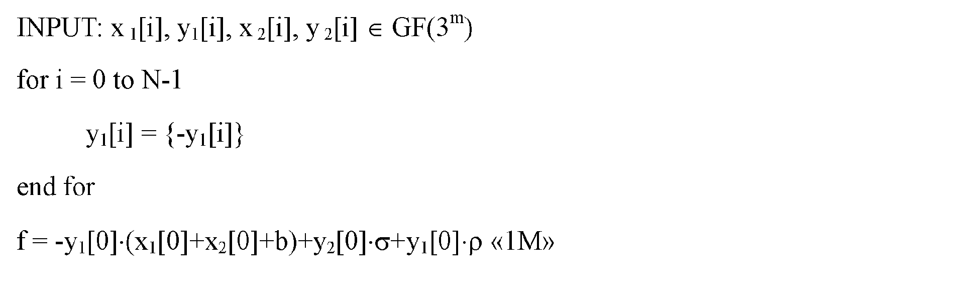


- As described above, if the improved ηT pairing calculation algorithm disclosed in the prior-
art literature 1 is simply extended to the multi-pairing calculation, 14M calculations are required for each value of i according to the formula (74), and 28M calculations are required for two values of i. - As described above, the prior-
art literature 2 discloses no method for efficient calculation of the product of a plurality of pairings. However, the prior-art literature 2 discloses an algorithm based on the loop unrolling. In the following, it will be shown that the calculation amount cannot be reduced more substantially than this embodiment even if the concept of the algorithm based on the loop unrolling disclosed in the prior-art literature 2 is extend to the multi-pairing calculation. - The above polynomial -{u[i]}2+y1[i]·y2[i]·σ-u[i]·ρ-ρ2 has to be calculated for each of different pairings for different values of i and has to be calculated {(m-1)/2}+1 times in the loops for j = 0 to (m-1)/2 for each of the pairings. According to the method according to this embodiment, the polynomials -{u[i]}2+y1[i]·y2[i]·σ-u[i]·ρ-ρ2 are separately determined for different pairings for different values of i, respectively, and the product thereof is determined. To the contrary, according to the concept based on the loop unrolling disclosed in the prior-
art literature 2, the product of a plurality of polynomials-{u[i]}2+y1[i]·y2[i]·σ-u[i]·ρ-ρ2 calculated in the loops for j = 0 to (m-1)/2 for the one of the pairings is determined. - The following is the algorithm based on the loop unrolling disclosed in the prior-
art literature 2 extended to the multi-pairing calculation (unpublished). Note that the following description is intended to explain the characteristics of this embodiment but not to show that the algorithm described below for comparison was able to be easily invented at the priority data of this application or at the time of application of the present invention.


- As described above, according to this algorithm, g1[0] and g2[0] for the same value i = 0 are determined according to the formulas (75) and (77), and then, the product thereof is determined according to the formula (74). And g1[i] and g2[i] for the same values i = 1, ..., N-1 are determined according to the formulas (75) and (77), and then, the product thereof is determined according to the formula (82). According to this algorithm, however, cubic calculations in the formulas (76) and (80) are needed. This is because, although one calculation of f = f3 would otherwise be performed for each of the loops for j = 0 to (m-1)/2, the algorithm based on the loop unrolling requires the cubic calculations of the formulas (76) and (80), which correspond to the one calculation of f = f3, to be performed for each value of i = 0, ..., N-1 in the loops, because each pair of loops for j is combined into one loop in the algorithm.
- According to the algorithm according to this embodiment, the cubic calculations are performed as f = f3 outside the loops for j = 0 to (m-1)/2, and therefore, the calculation amount can be reduced compared with the algorithm that extends the concept of the loop unrolling to the multi-pairing calculation.
- The first embodiment concerns a case where N is an even number equal to or greater than 4. A modification of the first embodiment described below concerns a case where N is an odd number equal to or greater than 5.
-
Fig. 11 is a diagram for illustrating a process in the case where N is an odd number equal to or greater than 5. In this modification, it is assumed that L = N-1. The following description will be focused only on differences from the first embodiment. - According to this modification of the first embodiment, after the processing in step S138 described in the first embodiment, the
control part 123 determines whether or not i = (N-1)-2 (step S159). If it is not determined that i = (N-1)-2, thecontrol part 123 sets i+2 as a new i and stores the setting in thememory 124, and the process returns to step S129 (step S140). - If it is determined that i = (N-1)-2, the
control part 123 sets i+2 as a new i and stores the setting in the memory 124 (step S160). - Then, the GF(36m) calculation part 122-1 reads y1[i], y2[i] and u[i] ∈ GF(3m) from the
memory 124, performs the following calculation
and stores the calculation result g[i] ∈ GF(36m) in the memory 124 (step S161). - Then, the GF(36m) calculation part 122-3 reads g ∈ GF(36m) and g[i] ∈ GF(36m) from the
memory 124, performs the following calculation
and stores the calculation result in thememory 124 as a new g ∈ GF(36m) (step S162). Then, the processing stages in step S141 and the following steps described in the first embodiment are performed. - Next, a second embodiment of the present invention will be described.
- The first embodiment is an example in which the present invention is applied to the part of calculation of g of the improved ηT pairing calculation algorithm. According to the second embodiment, the present invention is applied to the parts of calculation of both f and g of the improved ηT pairing calculation algorithm. This allows further reduction of the calculation amount.
- According to this embodiment, K = 4, p = 3, d = 6, m is an odd number equal to or greater than 1, N is an even number equal to or greater than 4, W = N, elements R(i, 0), R(i, 1), R(i, 2) and R(i, 3) of the finite field GF(pm) are affine coordinate points X1[i], Y1[i], X2[i] and Y2[i] ∈ GF(pm), respectively, of two points P(X1[i], Y1[i]) and Q(X2[i], Y2[i]) on the elliptic curve E defined on the finite field GF(pm), the calculation e(R(i, 0), ..., R(i, K-1)) is a pairing calculation e(P(X1[i], Y1[i]), Q(X2[i], Y2[i])), and the calculation Πi=0 N-1e(R(i, 0), ..., R(i, K-1)) is a multi-pairing calculation Πi=0 N-1e(P(X1[i], Y1[i]), Q(X2[i], Y2[i])). Furthermore, according to this embodiment, the elliptic curve is the supersingular elliptic curve Eb expressed by the formula (10) (b = -1 or 1). Furthermore, the extension field calculation according to this embodiment is a calculation that determines polynomials that express elements of the sixth-order extension field GF(36m) of the finite field GF(3m)


-
Figs. 12 and13 are block diagrams for illustrating a basic configuration of a finitefield calculation part 220 according to the second embodiment. - A finite field calculation apparatus according to the second embodiment is the finite field calculation apparatus shown in
Fig. 2A with the finitefield calculation part 20 replaced with the finitefield calculation part 220 shown inFigs. 12 and13 . The following description will be focused only on the configuration of the finitefield calculation part 220. - As shown in
Figs. 12 and13 , the finitefield calculation part 220 according to this embodiment has GF(3m) calculation parts 121-1 to 121-4 that perform a calculation over the finite field GF(3m), GF(36m) calculation parts 122-1 to 122-5 and 122-9 that perform a calculation over the sixth-order extension field GF(36m) of the finite field GF(3m), GF(36m) calculation parts 222-1 to 222-5, acontrol part 123, amemory 124 and a GF(3)calculation part 125 that performs a calculation over the finite field GF(3). - The finite
field calculation part 220 is a special device that comprises a well-known or dedicated computer having a CPU, a RAM and a ROM, for example, and a special program. For example, the GF(36m) calculation parts 222-1 to 222-5 are functional parts that are implemented by a predetermined program read in by the CPU. At least a part of the finitefield calculation part 220 may be formed by an integrated circuit. -
Figs. 14 to 15 are diagrams for illustrating a process according to the second embodiment. In the following, the process according to the second embodiment will be described with reference to these drawings. - First, the processing stages in steps S101 to S105 described in the first embodiment are performed. Note that, as in the first embodiment, the processing stages in steps S102 to S105 are unnecessary when b = -1.
- Then, the GF(36m) calculation part 222-1 (first calculation part or sixth calculation part) reads x1[0], y1[0], x2[0] and y2[0] ∈ GF(3m) (i3 = 0) from the
memory 124, performs the following calculation over the sixth-order extension field GF(36m)
and stores the calculation result f[0] ∈ GF(36m) in the memory 124 (step S206). - Then, the GF(36m) calculation part 222-1 (second calculation part or seventh calculation part) reads x1[1], y1[1], x2[1] and y2[1] ∈ GF(3m) (i4 = 1) from the
memory 124, performs the following calculation over the sixth-order extension field GF(36m)
and stores the calculation result f[1] ∈ GF(36m) in the memory 124 (step S207). - Then, the GF(36m) calculation part 222-3 (third calculation part or eighth calculation part) reads the calculation results f[0] ∈ GF(36m) and f[1] ∈ GF(36m) from the
memory 124, performs the following calculation
and stores the calculation result f ∈ GF(36m) in the memory 124 (step S208). Note that the GF(36m) calculation part 222-3 determines a product f[0]·f[1] ∈ GF(36m) without performing any calculation that involves as operands the terms, being previously determined to be 0 ∈ GF(pm), of the calculation result f[0] and/or the calculation result f[1]. - Then, the
control part 123 sets i = 2 and stores the setting in the memory 124 (step S209). - Then, the GF(36m) calculation part 222-1 reads y1[i], y2[i], x2[i] and y2[i] ∈ GF(3m) (i3 = i) from the
memory 124, performs the following calculation
and stores the calculation result g[i] ∈ GF(36m) in the memory 124 (step S210). - In addition, the GF(36m) calculation part 222-2 reads y1[i+1], y2[i+1], x2[i+1] and y2[i+1] ∈ GF(3m) (i4 = i+1) from the
memory 124, performs the following calculation
and stores the calculation result f[i+1] ∈ GF(36m) in the memory 124 (step S211). - Then, the GF(36m) calculation part 222-3 reads the calculation results f[i] ∈ GF(36m) and f[i+1] ∈ GF(36m) from the
memory 124, performs the following calculation
and stores the calculation result f[i]·f[i+1] ∈ GF(36m) in the memory 124 (step S212). Note that the GF(36m) calculation part 222-3 determines a product f[i]·f[i+1] ∈ GF(36m) without performing any calculation that involves as operands the terms, being previously determined to be 0 ∈ GF(pm), of the calculation result f[i] and/or the calculation result f[i+1]. - Then, the GF(36m) calculation part 222-4 (fourth calculation part or ninth calculation part) reads f ∈ GF(36m) and f[i]·f[i+1] ∈ GF(36m) from the
memory 124, performs the following calculation
and stores the calculation result in thememory 124 as a new f ∈ GF(36m) (step S213). - Then, the
control part 123 determines whether or not i = N-2 (step S214). If it is not determined that i = N-2, the control part 214 sets i+2 as a new i and stores the setting in thememory 124, and the process returns to step S210 (step S215). - If it is determined that i = N-2, the processing stages in step S112 and the following steps in the first embodiment are performed.
- As described above, according to this embodiment, in addition to the improved calculation of g[i] and g[i+1] described in the first embodiment, the following polynomials are determined.



- Note that the coefficients of the terms of the indeterminate elements ρ2 ∈ GF(p6m), ρ·σ ∈ GF(p6m) and ρ2·σ ∈ GF(p6m) of the polynomials (95) and (96) that express the sixth-order extension field GF(36m) are previously determined to be 0. Since the product of such polynomials is calculated in advance, the terms whose coefficients are previously determined to be 0 do not have to be calculated, and therefore, the number of multiplications can be reduced.
- The second embodiment concerns a case where N is an even number equal to or greater than 4. A modification of the second embodiment described below concerns a case where N is an odd number equal to or greater than 5.
-
Fig. 16 is a diagram for illustrating a process in the case where N is an odd number equal to or greater than 5. In this modification, it is assumed that L = N-1. The following description will be focused only on differences from the second embodiment. - According to this modification of the second embodiment, after the processing in step S213 described in the second embodiment, the
control part 123 determines whether or not i = (N-1)-2 (step S254). If it is not determined that i = (N-1)-2, thecontrol part 123 sets i+2 as a new i and stores the setting in thememory 124, and the process returns to step S210 (step S215). - If it is determined that i = (N-1)-2, the
control part 123 sets i+2 as a new i and stores the setting in the memory 124 (step S255). - Then, the GF(36m) calculation part 222-1 reads y1[i], y2[i], x2[i] and y2[i] ∈ GF(3m) (i3 = i) from the
memory 124, performs the following calculation
and stores the calculation result g[i] ∈ GF(36m) in the memory 124 (step S256). - Then, the GF(36m) calculation part 222-4 reads f ∈ GF(36m) and f[i] ∈ GF(36m) from the
memory 124, performs the following calculation
and stores the calculation result in thememory 124 as a new f ∈ GF(36m) (step S257). Then, the processing stages in step S112 and the following steps described in the first embodiment are performed. - Next, a third embodiment of the present invention will be described.
- The first embodiment is an example in which the present invention is applied to the part of calculation of g of the improved ηT pairing calculation algorithm. According to the second embodiment, the present invention is applied to only the part of calculation of f of the improved ηT pairing calculation algorithm.
- According to this embodiment, K = 4, p = 3, d = 6, m is an odd number equal to or greater than 1, N is an even number equal to or greater than 4, L = N, elements R(i, 0), R(i, 1), R(i, 2) and R(i, 3) of the finite field GF(pm) are affine coordinate points X1[i], Y1[i], X2[i] and Y2[i] ∈ GF(pm), respectively, of two points P(X1[i], Y1[i]) and Q(X2[i], Y2[i]) on the elliptic curve E defined on the finite field GF(pm), the calculation e(R(i, 0), ..., R(i, K-1)) is a pairing calculation e(P(X1[i], Y1[i]), Q(X2[i], Y2[i])), and the calculation Πi=0 N-1e(R(i, 0), ..., R(i, K-1)) is a multi-pairing calculation Πi=0 N-1e(P(X1[i], Y1[i]), Q(X2[i], Y2[i])). Furthermore, according to this embodiment, the elliptic curve is the supersingular elliptic curve Eb expressed by the formula (10) (b = -1 or 1). Furthermore, the extension field calculation according to this embodiment is a calculation that determines a polynomial that expresses elements of the sixth-order extension field GF(36m) of the finite field GF(3m)

where the affine coordinate points X1[i], Y1[i], X2[i] and Y2[i] input to the input part or the images thereof are represented by x1[i], y1[i], x2[i] and y2[i], respectively, u[i] = x1[i]+x2[i]+c ∈ GF(3m), the indeterminate element σ is a root of the irreducible polynomial σ2+1 = 0 whose coefficients are elements of the finite field GF(3m), and the indeterminate element p is a root of the irreducible polynomial ρ3-ρ - b = 0. The following description will be focused mainly on differences from the first embodiment, and descriptions of things common to those in the first embodiment will be omitted. -
Figs. 17 and18 are block diagrams for illustrating a basic configuration of a finitefield calculation part 320 according to the third embodiment.
A finite field calculation apparatus according to the third embodiment is the finite field calculation apparatus shown inFig. 2A with the finitefield calculation part 20 replaced with the finitefield calculation part 320 shown inFigs. 17 and18 . The following description will be focused only on the configuration of the finitefield calculation part 320. - As shown in
Figs. 17 and18 , the finitefield calculation part 320 according to this embodiment has GF(3m) calculation parts 121-1 to 121-4 that perform a calculation over the finite field GF(3m), GF(36m) calculation parts 122-1 to 122-5 and 122-9 that perform a calculation over the sixth-order extension field GF(36m) of the finite field GF(3m), GF(36m) calculation parts 222-1 to 222-5, GF(36m) calculation parts 322-1 and 322-2, acontrol part 123, amemory 124 and a GF(3)calculation part 125 that performs a calculation over the finite field GF(3). - The finite
field calculation part 320 is a special device that comprises a well-known or dedicated computer having a CPU, a RAM and a ROM, for example, and a special program. For example, the GF(36m) calculation parts 322-1 and 322-2 are functional parts that are implemented by a predetermined program read in by the CPU. At least a part of the finitefield calculation part 320 may be formed by an integrated circuit. -
Figs. 19 to 20 are diagrams for illustrating a process according to the third embodiment. In the following, the process according to the third embodiment will be described with reference to these drawings. - First, the processing stages in steps S101 to S105 and S206 to S215 described in the second embodiment (
Figs. 14 and15 ), and the processing stages in steps S112 to S118 described in the first embodiment are performed. Note that, as in the first embodiment, the processing stages in steps S102 to S105 are unnecessary when b = -1. If it is determined in step S117 that i = N-1, then, the GF(36m) calculation part 322-1 reads y1[0] ∈ GF(3m), y2[0] ∈ GF(3m) and u[0] ∈ GF(3m) (i1 = 0) from thememory 124, performs the following calculation
and stores the calculation result g ∈ GF(36m) in the memory 124 (step S319). - Then, the GF(36m) calculation part 322-1 reads y1[1] ∈ GF(3m), y2[1] ∈ GF(3m) and u[1] ∈ GF(3m) (i1 = 1) from the
memory 124, performs the following calculation
and stores the calculation result g' ∈ GF(36m) in thememory 124. Furthermore, the GF(36m) calculation part 322-2 reads g ∈ GF(36m) and g' ∈ GF(36m) from thememory 124, performs the following calculation
and stores the calculation result in thememory 124 as a new g (step S321). - Then, the
control part 123 sets i = 2 and stores the setting in the memory 124 (step S128). - Then, the GF(36m) calculation part 322-1 reads y1[i] ∈ GF(3m), y2[i] ∈ GF(3m) and u[i] ∈ GF(3m) (i1 = i) from the
memory 124, performs the following calculation
and stores the calculation result in thememory 124 as a new g' ∈ GF(36m) (step S329). - Then, the GF(36m) calculation part 322-2 reads the calculation results g ∈ GF(36m) and g' ∈ GF(36m) from the
memory 124, performs the following calculation
and stores the calculation result in thememory 124 as a new g (step S330).
Then, the processing stages in step S133 and the following steps in the first embodiment are performed. - Note that the present invention is not limited to the embodiments described above. For example, in the embodiments described above, i1 = 0 and i2 = 1, i1 = i and i2 = i+1, i3 = 0 and i4 = 1, and i3 = i and i4 = i+1. However, other values of i1, i2, i3 and i4 ∈ {0, ..., N-1} can also be used as far as i1 differs from i2, and i3 differs from i4. That is, a loop process can be performed in which the series of processing stages performed by the first calculation part, the second calculation part and the third calculation part is performed L/2 times while changing i1 and i2 in such a manner that each element of a subset including L (which represents an even number) different elements of the set {0, ..., N-1} is used one time as i1 or i2, and the series of processing stages performed by the sixth calculation part, the seventh calculation part and the eighth calculation part can be performed W/2 times while changing i3 and i4 in such a manner that each element of a subset comprising W (which represents a positive even number) different elements of the set {0, ..., N-1} is used one time as i3 or i4. In other words, each element of a subset including L (which represents an even number) different elements of the set {0, ..., N-1} is selected one time as i1 or i2, and first processing stages, each of which includes processing stages performed by the first calculation part, the second calculation part and the third calculation part are performed one time for each pair of selected i1 and i2, thereby performing the first processing stages for the L/2 pairs (i1, i2), respectively. And, each element of a subset comprising W (which represents a positive even number) different elements of the set {0, ..., N-1} is selected one time as i3 or i4, and second processing stages, each of which includes processing stages performed by the sixth calculation part, the seventh calculation part and the eighth calculation part one time for each pair of selected i3 and i4, thereby performing the second processing stages for the W/2 pairs (i3, i4), respectively.
- Furthermore, with regard to the embodiments described above, configurations in which N is an even number equal to or greater than 4 and L = N and/or W = N and in which N is an odd number equal to or greater than 5 and L = N-1 and/or W = N-1 have been described. However, other positive even numbers smaller than N may be L and/or W. In that case, the processing for i to which the method according to the present invention is not applied can be performed by repeating the cumulative calculation in steps S161 and S162 shown in
Fig. 11 or steps S256 and S257 shown inFig. 16 .
In addition, L may not be equal to W. N may assume 2 or 3. In that case, the processing stages in steps S108 to S111 and S113 inFig. 7 , the processings in steps S128 to S140 inFig. 9 , the processing stages in steps S128 to S159 inFig. 11 , the processing stages in steps S209 to S215 inFig. 15 , and the processing stages in steps S209 to S215 and S254 inFig. 16 are unnecessary. - In the embodiments described above, it is assumed that the parameters, such as b, are previously set. However, the parameters may be input to the apparatus.
- In the embodiments described above, it is assumed that the product poly(R(i1, 0), ..., R(i1, K-1))·poly(R(i2, 0), ..., R(i2, K-1)) is determined without performing any calculation that involves as operands the terms, being previously determined to be 0 ∈ GF(pm), of the polynomial poly(R(i1, 0), ..., R(i1, K-1)) and/or the polynomial poly(R(i2, 0), ..., R(i2, K-1)). However, a calculation that involves as operands some of these terms that are previously determined to be 0 ∈ GF(pm) may be performed.
- Furthermore, in the embodiments described above, the present invention is applied to the improved ηT pairing calculation algorithm of
characteristic 3. However, the present invention may be applied to other pairing calculations in characteristic 3, pairing calculations in characteristic 2, or pairing calculations in other characteristics. - The processings described above can be performed not only sequentially in the order described above but also in parallel with each other or individually as required or depending on the processing power of the apparatus that performs the processings. Furthermore, of course, other various modifications can be appropriately made to the processings without departing form the spirit of the present invention.
- In the case where the configurations described above are implemented by a computer, the specific processings of the apparatuses are described in a program. The computer executes the program to implement the processings described above.
- The program that describes the specific processings can be recorded in a computer-readable recording medium. The computer-readable recording medium may be any type of recording medium, such as a magnetic recording device, an optical disk, a magneto-optical recording medium and a semiconductor memory.
- The program may be distributed by selling, transferring or lending a portable recording medium, such as a DVD and a CD-ROM, in which the program is recorded, for example. Alternatively, the program may be distributed by storing the program in a storage device in a server computer and transferring the program from the server computer to other computers via a network.
- The computer that executes the program first temporarily stores, in a storage device thereof, the program recorded in a portable recording medium or transferred from a server computer, for example. Then, when performing the processings, the computer reads the program from the recording medium and performs the processings according to the read program. In an alternative implementation, the computer may read the program directly from the portable recording medium and perform the processings according to the program. As a further alternative, the computer may perform the processings according to the program each time the computer receives the program transferred from the server computer. As a further alternative, the processings described above may be performed on an application service provider (ASP) basis, in which the server computer does not transmit the program to the computer, and the processings are implemented only through execution instruction and result acquisition. The programs according to the embodiments of the present invention include a quasi-program, which is information processed by a computer (data or the like that is not a direct instruction to a computer but has a property that defines the processings performed by the computer).
- Industrial applications of the present invention include cryptographic applications that use a multi-pairing calculation, such as the inner product predicate encryption.
-
- 1
- finite field calculation apparatus
- 10
- input part
- 30
- output part
- 20, 120, 220, 320
- finite field calculation part
Claims (46)
- A finite field calculation apparatus, comprising:an input part adapted to accept N*K elements R(i, k) ∈ GF(pm) of a finite field GF(pm) where N ≥ 2, K ≥ 1, i ∈ {0, ..., N-1}, k ∈ {0, ..., K-1}, p represents a prime number, and m represents an integer equal to or greater than 1;a finite field calculation part adapted to perform a calculation Πi=0 N-1e(R(i, 0), ..., R(i, K-1)) where e(R(i, 0), ..., R(i, K-1)) represents a calculation of K elements R(i, 0), ..., R(i, K-1) ∈ GF(pm) of the finite field GF(pm) over a finite field; andan output part adapted to output a result of the calculation performed by the finite field calculation part,wherein the calculation e(R(i, 0), ... ,R(i, K-1)) over the finite field includes an extension field calculation over a d-th-order extension field GF(pd·m) of the finite field GF(pm) where d ≥ 2,the extension field calculation is a calculation that maps images over the finite field GF(pm) that depend on one or more input elements R(i, k) ∈ {R(i, 0), ..., R(i, K-1)} of the finite field GF(pm) and/or the elements R(i, k) ∈ {R(i, 0), ..., R(i, K-1)} of the finite field GF(pm) to a polynomial poly(R(i, 0), ..., R(i, K-1)) ∈ GF(pd·m) that expresses an element of the d-th-order extension field GF(pd·m),the polynomial poly(R(i, 0), ..., R(i, K-1)) ∈ GF(pd·m) is a polynomial having d terms, coefficients of the d terms include coefficients ah of some terms h ∈ {0, ..., d-1} and coefficients ar of predetermined some terms r ∈ {0, ..., d-1} (r ≠ h), the coefficients ah are the images over the finite field GF(pm) that depend on one or more input elements R(i, k) of the finite field GF(pm) and/or the elements R(i, k) of the finite field GF(pm), and the coefficients ar are previously determined to be 0 ∈ GF(pm), andthe finite field calculation part includes:a first calculation part adapted to receive, for any i1 ∈ {0, ..., N-1}, images over the finite field GF(pm) that depend on one or more elements R(i1, k) of the finite field GF(pm) and/or the elements R(i1, k) of the finite field GF(pm) and to perform the extension field calculation therefor to obtain a polynomial poly(R(i1, 0), ..., R(i1, K-1)) ∈ GF(pd·m);a second calculation part adapted to receive, for any i2 ∈ {0, ..., N-1} (i2 ≠ i1), images over the finite field GF(pm) that depend on one or more elements R(i2, k) of the finite field GF(pm) and/or the elements R(i2, k) of the finite field GF(pm) and to perform the extension field calculation therefor to obtain a polynomial poly(R(i2, 0), ..., R(i2, K-1)) ∈ GF(pd·m);a third calculation part adapted to receive the polynomial poly(R(i1, 0), ..., R(i1, K-1)) and the polynomial poly(R(i2, 0), ..., R(i2, K-1)) and calculate product thereof as poly(R(i1, 0), ..., R(i1, K-1))·poly(R(i2, 0), ..., R(i2, K-1)) ∈ GF(pd·m);a control part adapted to select each element of a subset including L different elements of the set {0, ..., N-1} one time as i1 or i2, where L represents an even number, and run first processing stages, each of which includes processing stages performed by the first calculation part, the second calculation part and the third calculation part , each of the first processing stages are performed one time for each pair of selected i1 and i2, to perform a loop process including the first processing stages for L/2 pairs of selected i1 and i2; anda fourth calculation part adapted to calculate Πi=0 N-1poly(R(i, 0), ..., R(i, K-1)) ∈ GF(pd·m) using products poly(R(i1, 0), ..., R(i1, K-1))·poly(R(i2, 0), ..., R(i2, K-1)) obtained by the first processing stages.
- The finite field calculation apparatus according to Claim 1, wherein the third calculation part determines the products poly(R(i1, 0), ..., R(i1, K-1))·poly(R(i2, 0), ..., R(i2, K-1)) without performing any calculation that involves as operands the terms, being previously determined to be 0 ∈ GF(pm), of said polynomial poly(R(i1, 0), ..., R(i1, K-1)) and/or the polynomial poly(R(i2, 0), ..., R(i2, K-1)).
- The finite field calculation apparatus according to Claim 1 or 2, wherein N is an even number, L = N, and the subset is the set {0, ..., N-1}.
- The finite field calculation apparatus according to Claim 1 or 2, wherein the control part runs, multiple times, the loop process including the L/2 first processing stages.
- The finite field calculation apparatus according to Claim 3, wherein the control part runs, multiple times, the loop process including the L/2 first processing stages.
- The finite field calculation apparatus according to Claim 1 or 2, wherein N ≥ 4, and
the fourth calculation part determines Πi=0 N-1poly(R(i, 0), ..., R(i, K-1)) ∈ GF(pd·m) using a multiplication value of the products poly(R(i1, 0), ..., R(i1, K-1))·poly(R(i2, 0), ..., R(i2, K-1)) obtained by the first processing stages. - The finite field calculation apparatus according to Claim 3, wherein N ≥ 4, and
the fourth calculation part determines Πi=0 N-1poly(R(i, 0), ..., R(i, K-1)) ∈ GF(pd·m) using a multiplication value of the products poly(R(i1, 0), ..., R(i1, K-1))·poly(R(i2, 0), ..., R(i2, K-1)) obtained by the first processing stages. - The finite field calculation apparatus according to Claim 4, wherein N ≥ 4, and
the fourth calculation part determines IIi=0 N-1poly(R(i, 0), ..., R(i, K-1)) ∈ GF(pd·m) using a multiplication value of the products poly(R(i1, 0), ..., R(i1, K-1))·poly(R(i2, 0), ..., R(i2, K-1)) obtained by the first processing stages. - The finite field calculation apparatus according to Claim 5, wherein N ≥ 4, and
the fourth calculation part determines Πi=0 N-1poly(R(i, 0), ..., R(i, K-1)) ∈ GF(pd·m) using a multiplication value of the products poly(R(i1, 0), ..., R(i1, K-1))·poly(R(i2, 0), ..., R(i2, K-1)) obtained by the first processing stages. - The finite field calculation apparatus according to Claim 6, wherein the fourth calculation part updates the multiplication value of the products poly(R(i1, 0), ..., R(i1, K-1))·poly(R(i2, 0), ..., R(i2, K-1)) that have been obtained at that point each time each of the first processing stages is performed.
- The finite field calculation apparatus according to Claim 7, wherein the fourth calculation part updates the multiplication value of the products poly(R(i1, 0), ..., R(i1, K-1))·poly(R(i2, 0), ..., R(i2, K-1)) that have been obtained at that point each time each of the first processing stages is performed.
- The finite field calculation apparatus according to Claim 8, wherein the fourth calculation part updates the multiplication value of the products poly(R(i1, 0), ..., R(i1, K-1))·poly(R(i2, 0), ..., R(i2, K-1)) that have been obtained at that point each time each of the first processing stages is performed.
- The finite field calculation apparatus according to Claim 9, wherein the fourth calculation part updates the multiplication value of the products poly(R(i1, 0), ..., R(i1, K-1))·poly(R(i2, 0), ..., R(i2, K-1)) that have been obtained at that point each time each of the first processing stages is performed.
- The finite field calculation apparatus according to Claim 1, wherein K = 4,
elements R(i, 0), R(i, 1), R(i, 2) and R(i, 3) of the finite field GF(pm) are affine coordinate points X1[i], Y1[i], X2[i] and Y2[i] ∈ GF(pm) of two points P(X1[i],Y1[i]) and Q(X2[i],Y2[i]) on an elliptic curve defined on the finite field GF(pm),
the calculation e(R(i, 0), ..., R(i, K-1)) is a pairing calculation e(P(X1[i], Y1[i]),Q(X2[i], Y2[i])), and
the calculation Πi=0 N-1e(R(i, 0), ..., R(i, K-1)) is a multi-pairing calculation Πi=0 N-1e(P(X1[i], Y1[i]), Q(X2[i], Y2[i])). - The finite field calculation apparatus according to Claim 14, wherein p = 3, d = 6,
the elliptic curve is Y2 = X3-X+b where b ∈ {-1,1},
the extension field calculation is a calculation that determines a polynomial poly(x1[i], y1[i], x2[i], y2[i]) = -{u[i]}2+y1[i]·y2[i]-σ-u[i]·ρ-ρ2 ∈ GF(36m) that expresses an element of a sixth-order extension field GF(36m) of the finite field GF(3m) where the affine coordinate points X1[i], Y1[i], X2[i] and Y2[i] input to the input part or the images thereof are represented by x1[i], y1[i], x2[i] and y2[i], u[i] = x1[i]+x2[i]+c ∈ GF(3m), an indeterminate element σ is a root of an irreducible polynomial σ2+1 = 0 a coefficient of which is an element of the finite field GF(3m), and an indeterminate element p is a root of an irreducible polynomial ρ3-ρ-b = 0,
the control part sets an initial value of c at b and adopts (c-b) mod 3 as a new value of c each time the loop process including the L/2 first processing stages is performed one time,
the polynomial poly(R(i1, 0), ..., R(i1, K-1)) is g[i1] = - {u[i1]}2y1[i1]·y2[i1]·σ-u[i1]·ρ-ρ2 ∈ GF(36m),
the polynomial poly(R(i2, 0), ..., R(i2, K-1)) is g[i2] =-{u[i2]}2+y1[i2]-y2[i2]·σ-u[i2]·ρ-ρ2 ∈ GF(36m),
the products poly(R(i1, 0), ..., R(i1, K-1))·poly(R(i2, 0), ..., R(i2, K-1)) are g[i1]·g[i2] ∈ GF(36m), and
the fourth calculation part calculates g = Πi=0 N-1poly(R(i, 0), ..., R(i, K-1)) ∈ GF(3d·m) using the products g[i1]·g[i2] obtained by the first processing stages. - The finite field calculation apparatus according to Claim 15, wherein the third calculation part determines the products poly(R(i1, 0), ..., R(i1, K-1))·poly(R(i2, 0), ..., R(i2, K-1)) without performing any calculation that involves as operands the terms, being previously determined to be 0 ∈ GF(pm), of the polynomial poly(R(i1, 0), ..., R(i1, K-1)) and/or the polynomial poly(R(i2, 0), ..., R(i2, K-1)).
- The finite field calculation apparatus according to Claim 15, wherein the control part performs an update processing each time each of the first processing stages is performed, the update processing including adopting -y1[i1] as a new y1[i1], adopting {x2[i1]}9 as a new x2[i1], adopting {y2[i1]}9 as a new y2[i1], adopting -y1[i2] as a new y1[i2], adopting {x2[i2]}9 as a new x2[i2], and adopting {y2[i2]}9 as a new y2[i2], and
the control part runs , multiple times, the loop process including the L/2 first processing stages. - The finite field calculation apparatus according to any one of Claims 15 to 17, wherein the finite field calculation part further includes a fifth calculation part adapted to perform a calculation of f = Πi=0 N-1(-y1[i]·(x1[i]+x2[i]+b)+y2[i]·σ+y1[i]·ρ) ∈ GF(36m) where x1[i] = X1[i], y1[i] = Y1[i], x2[i] = X2[i] and y2[i] = Y2[i] if b = -1 or x1[i] = X1[i], y1[i] = -Y1[i], x2[i] = X2[i] and y2[i] = Y2[i] if b = 1, and
a processing performed by the fifth calculation part is a processing performed before the first processing stages are performed for the first time. - The finite field calculation apparatus according to Claim 18, wherein the finite field calculation part further includes:a tenth calculation part adapted to calculate a product f·g ∈ GF(36m) of f obtained by the fifth calculation part and g obtained by the fourth calculation part as a new f; andan eleventh calculation part adapted to calculate a cube f3 ∈ GF(36m) of f obtained by the tenth calculation part as a new f, andprocessing stages performed by the tenth calculation part and the eleventh calculation part are performed each time the loop process is performed one time.
- The finite field calculation apparatus according to Claim 18, wherein N ≥ 4, and
the fifth calculation part includes:a sixth calculation part adapted to perform, for any i3 ∈ {0, ..., N-1}, a calculation of f[i3] =-y1[i3]·(x1[i3]+x2[i3]+b)+y2[i3]·σ+y1[i3]·ρ ∈ GF(36m);a seventh calculation part adapted to perform, for any i4 ∈ {0, ..., N-1} (i4 ≠ i3), a calculation of f[i4] = -y1[i4]·(x1[i4]+x2[i4]+b)+y2[i4]·σ+y1[i4]·ρ ∈ GF(3 6m);an eighth calculation part adapted to receive f[i3] and f[i4], and calculate the product thereof f[i3]·f[i4] ∈ GF(3d·m);a second control part adapted to select each element of a subset including W different elements of the set {0, ..., N-1} one time as i3 or i4, where W represents a positive even number, and runs W/2 second processing stages , each of which includes processing stages performed by the sixth calculation part, the seventh calculation part and the eighth calculation part for each pair of selected i3 and i4; anda ninth calculation part adapted to calculate f = Πi=0 N-1(-y1[i]·(x1[i]+x2[i]+b)+y2[i]·σ+y1[i]·ρ) ∈ GF(36m) using a multiplication value of the products f[i3]·f[i4] obtained by the second processing stages. - The finite field calculation apparatus according to Claim 20, wherein the finite field calculation part further includes:a tenth calculation part adapted to calculate a product f·g ∈ GF(36m) of f obtained by the fifth calculation part and g obtained by the fourth calculation part as a new f; andan eleventh calculation part adapted to calculate a cube f3 ∈ GF(36m) of f obtained by the tenth calculation part as a new f, andprocessing stages performed by the tenth calculation part and the eleventh calculation part are performed each time the loop process is performed one time.
- The finite field calculation apparatus according to Claim 14, wherein p = 3, d = 6,
the elliptic curve is Y2 = X3-X+b where b ∈ {-1,1},
the extension field calculation is a calculation that determines a polynomial poly(x1[i], y1[i], x2[i], y2[i]) = -y1[i]·(x1[i]+x2[i]+b)+y2[i]·σ+y1[i]·ρ ∈ GF(36m) that expresses an element of a sixth-order extension field GF(36m) of the finite field GF(3m) where the affine coordinate points X1[i], Y1[i], X 2[i] and Y2[i] input to the input part or the images thereof are represented by x1[i], y1[i], x2[i] and y2[i], an indeterminate element σ is a root of an irreducible polynomial σ2+1 = 0 a coefficient of which is an element of the finite field GF(3m), and an indeterminate element p is a root of an irreducible polynomial ρ3-ρ-b = 0. - A finite field calculation method for a finite field calculation apparatus that comprises an input part, a finite field calculation part and an output part, comprising:(A) a step of accepting N*K elements R(i, k) ∈ GF(pm) of a finite field GF(pm) by the input part where N ≥ 2, K ≥ 1, i ∈ {0, ..., N-1}, k ∈ {0, ..., K-1}, p represents a prime number, and m represents an integer equal to or greater than 1;(B) a step of performing a calculation Πi=0 N-1e(R(i, 0), ..., R(i, K-1)) by the finite field calculation part, where e(R(i, 0), ..., R(i, K-1)) represents a calculation of K elements R(i, 0), ..., R(i, K-1) ∈ GF(pm) of the finite field GF(pm) over a finite field; and(C) a step of outputting, from the output part, a result of the calculation in the step (B),
wherein the calculation e(R(i, 0), ... ,R(i, K-1)) over the finite field includes an extension field calculation over a d-th-order extension field GF(pd·m) of the finite field GF(pm) where d ≥ 2,
the extension field calculation is a calculation that maps images over the finite field GF(pm) that depend on one or more input elements R(i, k) ∈ {R(i, 0), ..., R(i, K-1)} of the finite field GF(pm) and/or the elements R(i, k) ∈ {R(i, 0), ..., R(i, K-1)} of the finite field GF(pm) to a polynomial poly(R(i, 0), ..., R(i, K-1)) ∈ GF(pd·m) that expresses an element of the d-th-order extension field GF(pd·m),
the polynomial poly(R(i, 0), ..., R(i, K-1)) ∈ GF(pd·m) is a polynomial having d terms, coefficients of the d terms include coefficients ah of some terms h ∈ {0, ..., d-1} and coefficients ar of predetermined some terms r ∈ {0, ..., d-1} (r ≠ h), the coefficients ah are the images over the finite field GF(pm) that depend on one or more input elements R(i, k) of the finite field GF(pm) and/or the elements R(i, k) of the finite field GF(pm), and the coefficients ar are previously determined to be 0 ∈ GF(pm),
the step (B) includes:(B-1) a step of inputting, for any i1 ∈ {0, ..., N-1}, images over the finite field GF(pm) that depend on one or more elements R(i1, k) of the finite field GF(pm) and/or the elements R(i1, k) of the finite field GF(pm) into a first calculation part of the finite field calculation part, and performing, by the first calculation part, the extension field calculation therefor to obtain a polynomial poly(R(i1, 0), ..., R(i1, K-1)) ∈ GF(pd·m);(B-2) a step of inputting, for any i2 ∈ {0, ..., N-1} (i2 ≠ i1), images over the finite field GF(pm) that depend on one or more elements R(i2, k) of the finite field GF(pm) and/or the elements R(i2, k) of the finite field GF(pm) into a second calculation part of the finite field calculation part, and performing, by the second calculation part, the extension field calculation therefor to obtain a polynomial poly(R(i2, 0), ..., R(i2, K-1)) ∈ GF(pd·m);(B-3) a step of inputting the polynomial poly(R(i1, 0), ..., R(i1, K-1)) and the polynomial poly(R(i2, 0), ..., R(i2, K-1)) into a third calculation part of the finite field calculation part, and calculating product thereof as poly(R(i1, 0), ..., R(i1, K-1))·poly(R(i2, 0), ..., R(i2, K-1)) ∈ GF(pd·m) by the third calculation part;(B-4) a step of calculating, by a fourth calculation part of the finite field calculation part, Πi=0 N-1poly(R(i, 0), ..., R(i, K-1)) ∈ GF(pd·m) using products poly(R(i1, 0), ..., R(i1, K-1))·poly(R(i2, 0), ..., R(i2, K-1)) obtained by first processing stages each of which includes the steps (B-1), (B-2) and (B-3), wherein
each element of a subset including L different elements of the set {0, ..., N-1} is selected one time as i1 or i2, where L represents an even number, and each of the first processing stages is performed one time for each pair of selected i1 and i2 to perform a loop process including the first processing stages for the L/2 pairs of selected i1 and i2, and
the step (B-4) includes a step of calculating Πi=0 N-1poly(R(i, 0), ..., R(i, K-1)) ∈ GF(pd·m) using products poly(R(i1, 0), ..., R(i1, K-1))·poly(R(i2, 0), ..., R(i2, K-1)) for the L/2 pairs. - The finite field calculation method according to Claim 23, wherein the step (B-3) includes a step of determining the products poly(R(i1, 0), ..., R(i1, K-1))·poly(R(i2, 0), ..., R(i2, K-1)) without performing any calculation that involves as operands the terms, being previously determined to be 0 ∈ GF(pm), of the polynomial poly(R(i1, 0), ..., R(i1, K-1)) and/or the polynomial poly(R(i2, 0), ..., R(i2, K-1)).
- The finite field calculation method according to Claim 23 or 24, wherein N is an even number, L = N, and the subset is the set {0, ..., N-1}.
- The finite field calculation method according to Claim 23 or 24, wherein the loop process including the L/2 first processing stages is performed multiple times.
- The finite field calculation method according to Claim 25, wherein the loop process including the L/2 first processing stages is performed multiple times.
- The finite field calculation method according to Claim 23 or 24, wherein N ≥ 4, and
the step (B-4) includes a step of determining Πi=0 N-1 poly(R(i, 0), ..., R(i, K-1)) ∈ GF(pd·m) using a multiplication value of the products poly(R(i1, 0), ..., R(i1, K-1))·poly(R(i2, 0), ..., R(i2, K-1)) obtained by the first processing stages. - The finite field calculation method according to Claim 25, wherein N ≥ 4, and
the step (B-4) includes a step of determining Πi=0 N-1poly(R(i, 0), ..., R(i, K-1)) ∈ GF(pd·m) using a multiplication value of the products poly(R(i1, 0), ..., R(i1, K-1))·poly(R(i2, 0), ..., R(i2, K-1)) obtained by the first processing stages. - The finite field calculation method according to Claim 26, wherein N ≥ 4, and
the step (B-4) includes a step of determining Πi=0 N-1poly(R(i, 0), ..., R(i, K-1)) ∈ GF(pd·m) using a multiplication value of the products poly(R(i1, 0), ..., R(i1, K-1))·poly(R(i2, 0), ..., R(i2, K-1)) obtained by the first processing stages. - The finite field calculation method according to Claim 27, wherein N ≥ 4, and
the step (B-4) includes a step of determining Πi=0 N-1poly(R(i, 0), ..., R(i, K-1)) ∈ GF(pd·m) using a multiplication value of the products poly(R(i1, 0), ..., R(i1, K-1))·poly(R(i2, 0), ..., R(i2, K-1)) obtained by the first processing stages. - The finite field calculation method according to Claim 28, wherein the step (B-4) includes a step of updating the multiplication value of the products poly(R(i1, 0), ..., R(i1, K-1))·poly(R(i2, 0), ..., R(i2, K-1)) that have been obtained at that point each time each of the first processing stages is performed.
- The finite field calculation method according to Claim 29, wherein the step (B-4) includes a step of updating the multiplication value of the products poly(R(i1, 0), ..., R(i1, K-1))·poly(R(i2, 0), ..., R(i2, K-1)) that have been obtained at that point each time each of the first processing stages is performed.
- The finite field calculation method according to Claim 30, wherein the step (B-4) includes a step of updating the multiplication value of the products poly(R(i1, 0), ..., R(i1, K-1))·poly(R(i2, 0), ..., R(i2, K-1)) that have been obtained at that point each time each of the first processing stages is performed.
- The finite field calculation method according to Claim 31, wherein the step (B-4) includes a step of updating the multiplication value of the products poly(R(i1, 0), ..., R(i1, K-1))·poly(R(i2, 0), ..., R(i2, K-1)) that have been obtained at that point each time each of the first processing stage is performed.
- The finite field calculation method according to Claim 23, wherein K = 4,
elements R(i, 0), R(i, 1), R(i, 2) and R(i, 3) of the finite field GF(pm) are affine coordinate points X1[i], Y1[i], X2[i] and Y2[i] ∈ GF(pm) of two points P(X1[i],Y1[i]) and Q(X2[i],Y2[i]) on an elliptic curve defined on the finite field GF(pm),
the calculation e(R(i, 0), ..., R(i, K-1)) is a pairing calculation e(P(X1[i], Y1[i]),Q(X2[i], Y2[i])), and
the calculation Πi=0 N-1e(R(i, 0), ..., R(i, K-1)) is a multi-pairing calculation Πi=0 N-1e(P(X1[i], Y1[i]), Q(X2[i], Y2[i])). - The finite field calculation method according to Claim 36, wherein p = 3, d = 6,
the elliptic curve is Y2 = X3-X+b where b ∈ {-1,1},
the extension field calculation is a calculation that determines a polynomial poly(x1[i], y1[i], X2[i], y2[i]) = -{u[i]}2+y1[i]-y2[i]·σ-u[i]·ρ-ρ2 ∈ GF(36m) that expresses an element of a sixth-order extension field GF(36m) of the finite field GF(3m) where the affine coordinate points X1[i], Y1[i], X2[i] and Y2[i] input to the input part or the images thereof are represented by x1[i], y1[i], x2[i] and y2[i], u[i] = x1[i]+x2[i]+c ∈ GF(3m), an indeterminate element σ is a root of an irreducible polynomial σ2+1 = 0 a coefficient of which is an element of the finite field GF(3m), and an indeterminate element p is a root of an irreducible polynomial ρ3-ρ-b = 0,
an initial value of c is set at b, (c-b) mod 3 is adopted as a new value of c each time the loop process including the L/2 first processing stages is performed one time,
the polynomial poly(R(i1, 0), ..., R(i1, K-1)) is g[i1] =-{u[i1]}2+y1[i1]-y2[i1]·σ-u[i1]·ρ-ρ2 ∈ GF(36m),
the polynomial poly(R(i2, 0), ..., R(i2, K-1)) is g[i2] =-{u[i2]}2+y1[i2]·y2[i2]·σ-u[i2]·ρ-ρ2 ∈ GF(36m),
the products poly(R(i1, 0), ..., R(i1, K-1))·poly(R(i2, 0), ..., R(i2, K-1)) are g[i1]·g[i2] ∈ GF(36m), and
the step (B-4) includes a step of calculating g = Πi=0 N-1poly(R(i, 0), ..., R(i, K-1)) ∈ GF(3d·m) using the products g[i1]·g[i2] obtained by the first processing stages. - The finite field calculation method according to Claim 37, wherein the step (B-3) includes a step of determining the products poly(R(i1, 0), ..., R(i1, K-1))·poly(R(i2, 0), ..., R(i2, K-1)) without performing any calculation that involves as operands the terms, being previously determined to be 0 ∈ GF(pm), of the polynomial poly(R(i1, 0), ..., R(i1, K-1)) and/or the polynomial poly(R(i2, 0), ..., R(i2, K-1)).
- The finite field calculation method according to Claim 37, wherein an update processing is performed each time each of the first processing stages is performed, the update processing including adopting - y1[i1] as a new y1[i1], adopting {x2[i1]}9 as a new x2[i1], adopting {y2[i1]}9 as a new y2[i1], adopting -y1[i2] as a new y1[i2], adopting {x2[i2]}9 as a new x2[i2], and adopting {y2[i2]}9 as a new y2[i2], and
the loop process including the L/2 first processing stages is performed multiple times. - The finite field calculation method according to any one of Claims 37 to 39, wherein the step (B) further includes:(B-5) a step of performing, by a fifth calculation part of the finite field calculation part, a calculation of f = Πi=0 N-1(-y1[i]·(x1[i]+x2[i]+b)+y2[i]·σ+y1[i]·ρ) ∈ GF(36m) where x1[i] = X1[i], y1[i] = Y1[i], x2[i] = X2[i] and y2[i] =Y2[i] if b = -1 or x1[i] = X1[i], y1[i]= -Y1[i], x2[i] = X2[i] and y2[i] =Y2[i] if b = 1, and
the step (B-5) is performed before the first processing stages are performed for the first time. - The finite field calculation method according to Claim 40, wherein the step (B) further includes:(B-10) a step of calculating, by a tenth calculation part of the finite field calculation part, a product f·g ∈ GF(36m) of f obtained in the step (B-5) and g obtained in the step (B-4) as a new f; and(B-11) a step of calculating, by an eleventh calculation part of the finite field calculation part, a cube f3 ∈ GF(36m) of f obtained in the step (B-6) as a new f, andprocessing stages performed in the steps (B-10) and (B-11) are performed each time the loop process is performed one time.
- The finite field calculation method according to Claim 40, wherein N ≥ 4, and
the step (B-5) includes:(B-6) a step of performing, by a sixth calculation part of the finite field calculation part, for any i3 ∈ {0, ..., N-1}, a calculation of f[i3] =-y1[i3]·(x1[i3]+x2[i3]+b)+y2[i3]·σ+y1[i3]·ρ ∈ GF(36m);(B-7) a step of performing, by a seventh calculation part of the finite field calculation part, for any i4 ∈ {0, ..., N-1} (i4 ≠ i3), a calculation of f[i4] = -y1[i4]·(x1[i4]+x2[i4]+b)+y2[i4]·σ+y1[i4]·ρ ∈ GF(36m);(B-8) a step of receiving f[i3] and f[i4] and calculating the product thereof f[i3]·f[i4] ∈ GF(3d·m) by an eighth calculation part of the finite field calculation part; and(B-9) a step of calculating, by a ninth calculation part of the finite field calculation part, f = Πi=0 N-1(-y1[i]·(x1[i]+x2[i]+b)+y2[i]·σ+y1[i]·ρ) ∈ GF(36m) using a multiplication value of the products f[i3]·f[i4] obtained by second processing stages each of which includes the steps (B-6), (B-7) and (B-8), and
each element of a subset including W different elements of the set {0, ..., N-1} is selected one time as i3 or i4, where W represents a positive even number, and each of the second processing stages is performed one time for each pair of selected i3 and i4, to perform the second processing stages for W/2 pairs (i3, i4). - The finite field calculation method according to Claim 42, wherein the step (B) further includes:(B-10) a step of calculating, by a tenth calculation part of the finite field calculation part, a product f·g ∈ GF(36m) of f obtained in the step (B-5) and g obtained in the step (B-4) as a new f; and(B-11) a step of calculating, by an eleventh calculation part of the finite field calculation part, a cube f3 ∈ GF(36m) of f obtained in the step (B-6) as a new f, andprocessings in the steps (B-10) and (B-11) are performed each time the loop process is performed one time.
- The finite field calculation method according to Claim 36, wherein p = 3, d = 6,
the elliptic curve is Y2 = X3-X+b where b ∈ {-1,1},
the extension field calculation is a calculation that determines a polynomial poly(x1[i], y1[i], x2[i], y2[i]) = -y1[i]·(x1[i]+x2[i]+b)+y2[i]·σ+y1[i]·ρ ∈ GF(36m) that expresses an element of a sixth-order extension field GF(36m) of the finite field GF(3m) where the affine coordinate points X1[i], Y1[i], X 2[i] and Y2[i] input to the input part or the images thereof are represented by x1[i], y1[i], x2[i] and y2[i], an indeterminate element σ is a root of an irreducible polynomial σ2+1 = 0 a coefficient of which is an element of the finite field GF(3m), and an indeterminate element p is a root of an irreducible polynomial ρ3-ρ-b = 0. - A program that makes a computer perform function of a finite field calculation apparatus according to Claim 1.
- A computer-readable recording medium that stores a program that makes a computer perform function of a finite field calculation apparatus according to Claim 1.
Applications Claiming Priority (2)
| Application Number | Priority Date | Filing Date | Title |
|---|---|---|---|
| JP2009106029 | 2009-04-24 | ||
| PCT/JP2010/057281 WO2010123117A1 (en) | 2009-04-24 | 2010-04-23 | Finite field calculation apparatus, finite filed calculation method, program, and recording medium |
Publications (3)
| Publication Number | Publication Date |
|---|---|
| EP2423905A1 true EP2423905A1 (en) | 2012-02-29 |
| EP2423905A4 EP2423905A4 (en) | 2013-10-16 |
| EP2423905B1 EP2423905B1 (en) | 2016-03-16 |
Family
ID=43011231
Family Applications (1)
| Application Number | Title | Priority Date | Filing Date |
|---|---|---|---|
| EP10767172.9A Not-in-force EP2423905B1 (en) | 2009-04-24 | 2010-04-23 | Apparatus, method, program and recording medium for computation of pairings over finite fields |
Country Status (6)
| Country | Link |
|---|---|
| US (1) | US8488780B2 (en) |
| EP (1) | EP2423905B1 (en) |
| JP (1) | JP5269188B2 (en) |
| KR (1) | KR101301139B1 (en) |
| CN (1) | CN102396010B (en) |
| WO (1) | WO2010123117A1 (en) |
Families Citing this family (5)
| Publication number | Priority date | Publication date | Assignee | Title |
|---|---|---|---|---|
| US9800407B2 (en) * | 2013-08-30 | 2017-10-24 | Qualcomm Incorporated | Methods and apparatuses for prime number generation and storage |
| JP6023728B2 (en) * | 2014-01-20 | 2016-11-09 | 日本電信電話株式会社 | Multi-pairing calculation device, multi-pairing calculation method, multi-pairing calculation program |
| JP6067596B2 (en) * | 2014-01-20 | 2017-01-25 | 日本電信電話株式会社 | Pairing arithmetic device, multi-pairing arithmetic device, program |
| JP6059287B2 (en) * | 2015-05-12 | 2017-01-11 | 日本電信電話株式会社 | Matrix triangulation device and program |
| CN106330429B (en) * | 2016-08-24 | 2019-08-06 | 中国信息安全测评中心 | Method and device for generating S-box of SM4 algorithm |
Family Cites Families (7)
| Publication number | Priority date | Publication date | Assignee | Title |
|---|---|---|---|---|
| SG42847A1 (en) * | 1993-05-05 | 1997-10-17 | Zunquan Liu | Device and method for data encryption |
| JP4181724B2 (en) * | 2000-03-03 | 2008-11-19 | 日本電気株式会社 | Re-encryption shuffle method and apparatus with certificate, re-encryption shuffle verification method and apparatus, input sentence string generation method and apparatus, and recording medium |
| KR100585119B1 (en) * | 2004-01-07 | 2006-06-01 | 삼성전자주식회사 | Encryption apparatus, encryption method and recording medium thereof |
| JP4630117B2 (en) * | 2005-04-25 | 2011-02-09 | 日本電信電話株式会社 | Multi-pairing calculation method, pairing comparison method, apparatus using the same, and program |
| JP4688886B2 (en) * | 2006-01-11 | 2011-05-25 | 三菱電機株式会社 | Elliptic curve encryption parameter generation apparatus, elliptic curve encryption system, and elliptic curve encryption parameter generation program |
| JP4856599B2 (en) * | 2007-07-25 | 2012-01-18 | 日本電信電話株式会社 | Pairing arithmetic device, program |
| JP5349261B2 (en) * | 2009-04-23 | 2013-11-20 | 三菱電機株式会社 | Cryptographic processing system, key generation device, key delegation device, encryption device, decryption device, cryptographic processing method, and cryptographic processing program |
-
2010
- 2010-04-23 CN CN201080016403.5A patent/CN102396010B/en not_active Expired - Fee Related
- 2010-04-23 JP JP2011510384A patent/JP5269188B2/en not_active Expired - Fee Related
- 2010-04-23 KR KR1020117023973A patent/KR101301139B1/en active Active
- 2010-04-23 WO PCT/JP2010/057281 patent/WO2010123117A1/en not_active Ceased
- 2010-04-23 US US13/258,840 patent/US8488780B2/en active Active
- 2010-04-23 EP EP10767172.9A patent/EP2423905B1/en not_active Not-in-force
Non-Patent Citations (9)
| Title |
|---|
| JEAN-LUC BEUCHAT ET AL: "A Comparison Between Hardware Accelerators for the Modified Tate Pairing over mathbbF_2<m> and mathbbF_3<m>", INTERNATIONAL ASSOCIATION FOR CRYPTOLOGIC RESEARCH,, vol. 20080317:140712, 17 March 2008 (2008-03-17), pages 1-28, XP061002784, [retrieved on 2008-03-17] * |
| JEAN-LUC BEUCHAT ET AL: "A Coprocessor for the Final Exponentiation of the eta_T Pairing in Characteristic Three", INTERNATIONAL ASSOCIATION FOR CRYPTOLOGIC RESEARCH,, vol. 20070214:110206, 14 February 2007 (2007-02-14), pages 1-15, XP061002247, [retrieved on 2007-02-14] * |
| JEAN-LUC BEUCHAT ET AL: "An Algorithm for the eta_T Pairing Calculation in Characteristic Three and its Hardware Implementation", INTERNATIONAL ASSOCIATION FOR CRYPTOLOGIC RESEARCH,, vol. 20070323:001825, 23 March 2007 (2007-03-23), pages 1-11, XP061002082, [retrieved on 2007-03-23] * |
| MASAAKI SHIRASE ET AL: "Universal Î T Pairing Algorithm over Arbitrary Extension Degree", 27 August 2007 (2007-08-27), INFORMATION SECURITY APPLICATIONS; [LECTURE NOTES IN COMPUTER SCIENCE], SPRINGER BERLIN HEIDELBERG, BERLIN, HEIDELBERG, PAGE(S) 1 - 15, XP019137130, ISBN: 978-3-540-77534-8 * paragraphs [02.3], [0003] * * |
| MOTOI YOSHITOMI ET AL: "Efficient Implementation of the Pairing on Mobilephones Using BREW", 27 August 2007 (2007-08-27), INFORMATION SECURITY APPLICATIONS; [LECTURE NOTES IN COMPUTER SCIENCE], SPRINGER BERLIN HEIDELBERG, BERLIN, HEIDELBERG, PAGE(S) 203 - 214, XP019137136, ISBN: 978-3-540-77534-8 * paragraphs [02.3] - [03.2] * * |
| PAULO S L M BARRETO ET AL: "Efficient Pairing Computation on Supersingular Abelian Varieties", INTERNATIONAL ASSOCIATION FOR CRYPTOLOGIC RESEARCH,, vol. 20050905:142955, 5 September 2005 (2005-09-05), pages 1-35, XP061001091, [retrieved on 2005-09-05] * |
| ROBERT RONAN ET AL: "Hardware Implementation of the eta_T Pairing in Characteristic 3", INTERNATIONAL ASSOCIATION FOR CRYPTOLOGIC RESEARCH,, vol. 20061103:162149, 27 October 2006 (2006-10-27), pages 1-16, XP061001977, [retrieved on 2006-10-27] * |
| See also references of WO2010123117A1 * |
| YUTO KAWAHARA ET AL: "Efficient Implementation of Tate Pairing on a Mobile Phone Using Java", 3 November 2006 (2006-11-03), COMPUTATIONAL INTELLIGENCE AND SECURITY; [LECTURE NOTES IN COMPUTER SCIENCE], SPRINGER BERLIN HEIDELBERG, BERLIN, HEIDELBERG, PAGE(S) 396 - 405, XP019165326, ISBN: 978-3-540-74376-7 * paragraph [0002] * * |
Also Published As
| Publication number | Publication date |
|---|---|
| WO2010123117A1 (en) | 2010-10-28 |
| US20120033805A1 (en) | 2012-02-09 |
| KR101301139B1 (en) | 2013-09-03 |
| KR20120038395A (en) | 2012-04-23 |
| CN102396010A (en) | 2012-03-28 |
| CN102396010B (en) | 2014-10-22 |
| EP2423905B1 (en) | 2016-03-16 |
| JPWO2010123117A1 (en) | 2012-10-25 |
| JP5269188B2 (en) | 2013-08-21 |
| US8488780B2 (en) | 2013-07-16 |
| EP2423905A4 (en) | 2013-10-16 |
Similar Documents
| Publication | Publication Date | Title |
|---|---|---|
| Liu et al. | Efficient Ring-LWE encryption on 8-bit AVR processors | |
| Koziel et al. | Fast hardware architectures for supersingular isogeny Diffie-Hellman key exchange on FPGA | |
| McIvor et al. | Hardware Elliptic Curve Cryptographic Processor Over $ rm GF (p) $ | |
| Wiener et al. | Faster attacks on elliptic curve cryptosystems | |
| JP5378579B2 (en) | Module reduction using folding | |
| EP1993086B1 (en) | Elliptical curve encryption parameter generation device, elliptical curve encryption calculation device, elliptical curve encryption parameter generation program, and elliptical curve encryption calculation program | |
| Bos | Constant time modular inversion | |
| EP2423905B1 (en) | Apparatus, method, program and recording medium for computation of pairings over finite fields | |
| EP1816624A1 (en) | Encryption computing device | |
| EP2045716A2 (en) | Exponentiation calculation apparatus and exponentiation calculation method | |
| Putranto et al. | Another concrete quantum cryptanalysis of binary elliptic curves | |
| Shah et al. | LUT‐based high‐speed point multiplier for Goldilocks‐Curve448 | |
| Beuchat et al. | Fast Architectures for the\eta_T Pairing over Small-Characteristic Supersingular Elliptic Curves | |
| US20120321075A1 (en) | Fault-resistant exponentiationi algorithm | |
| Yasuda et al. | Computational hardness of IFP and ECDLP | |
| Sakamoto et al. | High-throughput bilinear pairing processor for server-side FPGA applications | |
| Kato et al. | Cyclic vector multiplication algorithm based on a special class of Gauss period normal basis | |
| Iyengar | Novel elliptic curve scalar multiplication algorithms for faster and safer public-key cryptosystems | |
| Seo et al. | Secure number theoretic transform and speed record for Ring-LWE encryption on embedded processors | |
| Di Tullio et al. | Elliptic curves of nearly prime order | |
| Erdem et al. | Efficient and Constant Time Modular Reduction With Generalized Mersenne Primes | |
| Oussama et al. | Software implementation of pairing based cryptography on FPGA | |
| Hashimoto et al. | An implementation of ecc with twisted montgomery curve over 32nd degree tower field on arduino uno | |
| Zarrah et al. | FPGA implementation of area-time efficient modular inversion over NIST prime fields | |
| Pillutla et al. | High-throughput area-delay-efficient systolic multiplier over GF (2m) for a class of trinomials |
Legal Events
| Date | Code | Title | Description |
|---|---|---|---|
| PUAI | Public reference made under article 153(3) epc to a published international application that has entered the european phase |
Free format text: ORIGINAL CODE: 0009012 |
|
| 17P | Request for examination filed |
Effective date: 20111124 |
|
| AK | Designated contracting states |
Kind code of ref document: A1 Designated state(s): AT BE BG CH CY CZ DE DK EE ES FI FR GB GR HR HU IE IS IT LI LT LU LV MC MK MT NL NO PL PT RO SE SI SK SM TR |
|
| DAX | Request for extension of the european patent (deleted) | ||
| A4 | Supplementary search report drawn up and despatched |
Effective date: 20130912 |
|
| RIC1 | Information provided on ipc code assigned before grant |
Ipc: G09C 1/00 20060101AFI20130906BHEP Ipc: H04L 9/30 20060101ALI20130906BHEP |
|
| 17Q | First examination report despatched |
Effective date: 20140722 |
|
| REG | Reference to a national code |
Ref country code: DE Ref legal event code: R079 Ref document number: 602010031238 Country of ref document: DE Free format text: PREVIOUS MAIN CLASS: G09C0001000000 Ipc: G06F0007720000 |
|
| GRAP | Despatch of communication of intention to grant a patent |
Free format text: ORIGINAL CODE: EPIDOSNIGR1 |
|
| RIC1 | Information provided on ipc code assigned before grant |
Ipc: H04L 9/30 20060101ALI20150223BHEP Ipc: G06F 7/72 20060101AFI20150223BHEP |
|
| INTG | Intention to grant announced |
Effective date: 20150325 |
|
| GRAP | Despatch of communication of intention to grant a patent |
Free format text: ORIGINAL CODE: EPIDOSNIGR1 |
|
| INTG | Intention to grant announced |
Effective date: 20150818 |
|
| GRAS | Grant fee paid |
Free format text: ORIGINAL CODE: EPIDOSNIGR3 |
|
| RIN1 | Information on inventor provided before grant (corrected) |
Inventor name: TAKAHASHI, GEN Inventor name: TAKEUCHI, KAKU Inventor name: KOBAYASHI, TETSUTARO |
|
| RAP1 | Party data changed (applicant data changed or rights of an application transferred) |
Owner name: NIPPON TELEGRAPH AND TELEPHONE COMPANY |
|
| GRAA | (expected) grant |
Free format text: ORIGINAL CODE: 0009210 |
|
| GRAT | Correction requested after decision to grant or after decision to maintain patent in amended form |
Free format text: ORIGINAL CODE: EPIDOSNCDEC |
|
| INTG | Intention to grant announced |
Effective date: 20160115 |
|
| RAP1 | Party data changed (applicant data changed or rights of an application transferred) |
Owner name: NIPPON TELEGRAPH AND TELEPHONE CORPORATION |
|
| AK | Designated contracting states |
Kind code of ref document: B1 Designated state(s): AT BE BG CH CY CZ DE DK EE ES FI FR GB GR HR HU IE IS IT LI LT LU LV MC MK MT NL NO PL PT RO SE SI SK SM TR |
|
| REG | Reference to a national code |
Ref country code: GB Ref legal event code: FG4D |
|
| REG | Reference to a national code |
Ref country code: CH Ref legal event code: EP |
|
| REG | Reference to a national code |
Ref country code: IE Ref legal event code: FG4D |
|
| REG | Reference to a national code |
Ref country code: AT Ref legal event code: REF Ref document number: 781769 Country of ref document: AT Kind code of ref document: T Effective date: 20160415 Ref country code: FR Ref legal event code: PLFP Year of fee payment: 7 |
|
| REG | Reference to a national code |
Ref country code: DE Ref legal event code: R096 Ref document number: 602010031238 Country of ref document: DE |
|
| REG | Reference to a national code |
Ref country code: NL Ref legal event code: MP Effective date: 20160316 |
|
| REG | Reference to a national code |
Ref country code: LT Ref legal event code: MG4D |
|
| PG25 | Lapsed in a contracting state [announced via postgrant information from national office to epo] |
Ref country code: FI Free format text: LAPSE BECAUSE OF FAILURE TO SUBMIT A TRANSLATION OF THE DESCRIPTION OR TO PAY THE FEE WITHIN THE PRESCRIBED TIME-LIMIT Effective date: 20160316 Ref country code: HR Free format text: LAPSE BECAUSE OF FAILURE TO SUBMIT A TRANSLATION OF THE DESCRIPTION OR TO PAY THE FEE WITHIN THE PRESCRIBED TIME-LIMIT Effective date: 20160316 Ref country code: NO Free format text: LAPSE BECAUSE OF FAILURE TO SUBMIT A TRANSLATION OF THE DESCRIPTION OR TO PAY THE FEE WITHIN THE PRESCRIBED TIME-LIMIT Effective date: 20160616 Ref country code: GR Free format text: LAPSE BECAUSE OF FAILURE TO SUBMIT A TRANSLATION OF THE DESCRIPTION OR TO PAY THE FEE WITHIN THE PRESCRIBED TIME-LIMIT Effective date: 20160617 |
|
| REG | Reference to a national code |
Ref country code: AT Ref legal event code: MK05 Ref document number: 781769 Country of ref document: AT Kind code of ref document: T Effective date: 20160316 |
|
| PG25 | Lapsed in a contracting state [announced via postgrant information from national office to epo] |
Ref country code: LT Free format text: LAPSE BECAUSE OF FAILURE TO SUBMIT A TRANSLATION OF THE DESCRIPTION OR TO PAY THE FEE WITHIN THE PRESCRIBED TIME-LIMIT Effective date: 20160316 Ref country code: BE Free format text: LAPSE BECAUSE OF NON-PAYMENT OF DUE FEES Effective date: 20160430 Ref country code: SE Free format text: LAPSE BECAUSE OF FAILURE TO SUBMIT A TRANSLATION OF THE DESCRIPTION OR TO PAY THE FEE WITHIN THE PRESCRIBED TIME-LIMIT Effective date: 20160316 Ref country code: LV Free format text: LAPSE BECAUSE OF FAILURE TO SUBMIT A TRANSLATION OF THE DESCRIPTION OR TO PAY THE FEE WITHIN THE PRESCRIBED TIME-LIMIT Effective date: 20160316 Ref country code: NL Free format text: LAPSE BECAUSE OF FAILURE TO SUBMIT A TRANSLATION OF THE DESCRIPTION OR TO PAY THE FEE WITHIN THE PRESCRIBED TIME-LIMIT Effective date: 20160316 |
|
| PG25 | Lapsed in a contracting state [announced via postgrant information from national office to epo] |
Ref country code: IS Free format text: LAPSE BECAUSE OF FAILURE TO SUBMIT A TRANSLATION OF THE DESCRIPTION OR TO PAY THE FEE WITHIN THE PRESCRIBED TIME-LIMIT Effective date: 20160716 Ref country code: PL Free format text: LAPSE BECAUSE OF FAILURE TO SUBMIT A TRANSLATION OF THE DESCRIPTION OR TO PAY THE FEE WITHIN THE PRESCRIBED TIME-LIMIT Effective date: 20160316 Ref country code: EE Free format text: LAPSE BECAUSE OF FAILURE TO SUBMIT A TRANSLATION OF THE DESCRIPTION OR TO PAY THE FEE WITHIN THE PRESCRIBED TIME-LIMIT Effective date: 20160316 |
|
| PG25 | Lapsed in a contracting state [announced via postgrant information from national office to epo] |
Ref country code: AT Free format text: LAPSE BECAUSE OF FAILURE TO SUBMIT A TRANSLATION OF THE DESCRIPTION OR TO PAY THE FEE WITHIN THE PRESCRIBED TIME-LIMIT Effective date: 20160316 Ref country code: ES Free format text: LAPSE BECAUSE OF FAILURE TO SUBMIT A TRANSLATION OF THE DESCRIPTION OR TO PAY THE FEE WITHIN THE PRESCRIBED TIME-LIMIT Effective date: 20160316 Ref country code: SK Free format text: LAPSE BECAUSE OF FAILURE TO SUBMIT A TRANSLATION OF THE DESCRIPTION OR TO PAY THE FEE WITHIN THE PRESCRIBED TIME-LIMIT Effective date: 20160316 Ref country code: SM Free format text: LAPSE BECAUSE OF FAILURE TO SUBMIT A TRANSLATION OF THE DESCRIPTION OR TO PAY THE FEE WITHIN THE PRESCRIBED TIME-LIMIT Effective date: 20160316 Ref country code: RO Free format text: LAPSE BECAUSE OF FAILURE TO SUBMIT A TRANSLATION OF THE DESCRIPTION OR TO PAY THE FEE WITHIN THE PRESCRIBED TIME-LIMIT Effective date: 20160316 Ref country code: CZ Free format text: LAPSE BECAUSE OF FAILURE TO SUBMIT A TRANSLATION OF THE DESCRIPTION OR TO PAY THE FEE WITHIN THE PRESCRIBED TIME-LIMIT Effective date: 20160316 Ref country code: PT Free format text: LAPSE BECAUSE OF FAILURE TO SUBMIT A TRANSLATION OF THE DESCRIPTION OR TO PAY THE FEE WITHIN THE PRESCRIBED TIME-LIMIT Effective date: 20160718 |
|
| REG | Reference to a national code |
Ref country code: CH Ref legal event code: PL |
|
| REG | Reference to a national code |
Ref country code: DE Ref legal event code: R097 Ref document number: 602010031238 Country of ref document: DE |
|
| PG25 | Lapsed in a contracting state [announced via postgrant information from national office to epo] |
Ref country code: IT Free format text: LAPSE BECAUSE OF FAILURE TO SUBMIT A TRANSLATION OF THE DESCRIPTION OR TO PAY THE FEE WITHIN THE PRESCRIBED TIME-LIMIT Effective date: 20160316 Ref country code: BE Free format text: LAPSE BECAUSE OF FAILURE TO SUBMIT A TRANSLATION OF THE DESCRIPTION OR TO PAY THE FEE WITHIN THE PRESCRIBED TIME-LIMIT Effective date: 20160316 |
|
| PLBE | No opposition filed within time limit |
Free format text: ORIGINAL CODE: 0009261 |
|
| STAA | Information on the status of an ep patent application or granted ep patent |
Free format text: STATUS: NO OPPOSITION FILED WITHIN TIME LIMIT |
|
| REG | Reference to a national code |
Ref country code: IE Ref legal event code: MM4A |
|
| PG25 | Lapsed in a contracting state [announced via postgrant information from national office to epo] |
Ref country code: CH Free format text: LAPSE BECAUSE OF NON-PAYMENT OF DUE FEES Effective date: 20160430 Ref country code: LI Free format text: LAPSE BECAUSE OF NON-PAYMENT OF DUE FEES Effective date: 20160430 Ref country code: DK Free format text: LAPSE BECAUSE OF FAILURE TO SUBMIT A TRANSLATION OF THE DESCRIPTION OR TO PAY THE FEE WITHIN THE PRESCRIBED TIME-LIMIT Effective date: 20160316 |
|
| 26N | No opposition filed |
Effective date: 20161219 |
|
| PG25 | Lapsed in a contracting state [announced via postgrant information from national office to epo] |
Ref country code: BG Free format text: LAPSE BECAUSE OF FAILURE TO SUBMIT A TRANSLATION OF THE DESCRIPTION OR TO PAY THE FEE WITHIN THE PRESCRIBED TIME-LIMIT Effective date: 20160616 |
|
| REG | Reference to a national code |
Ref country code: FR Ref legal event code: PLFP Year of fee payment: 8 |
|
| PG25 | Lapsed in a contracting state [announced via postgrant information from national office to epo] |
Ref country code: IE Free format text: LAPSE BECAUSE OF NON-PAYMENT OF DUE FEES Effective date: 20160423 Ref country code: SI Free format text: LAPSE BECAUSE OF FAILURE TO SUBMIT A TRANSLATION OF THE DESCRIPTION OR TO PAY THE FEE WITHIN THE PRESCRIBED TIME-LIMIT Effective date: 20160316 |
|
| REG | Reference to a national code |
Ref country code: FR Ref legal event code: PLFP Year of fee payment: 9 |
|
| PG25 | Lapsed in a contracting state [announced via postgrant information from national office to epo] |
Ref country code: CY Free format text: LAPSE BECAUSE OF FAILURE TO SUBMIT A TRANSLATION OF THE DESCRIPTION OR TO PAY THE FEE WITHIN THE PRESCRIBED TIME-LIMIT Effective date: 20160316 Ref country code: HU Free format text: LAPSE BECAUSE OF FAILURE TO SUBMIT A TRANSLATION OF THE DESCRIPTION OR TO PAY THE FEE WITHIN THE PRESCRIBED TIME-LIMIT; INVALID AB INITIO Effective date: 20100423 |
|
| PG25 | Lapsed in a contracting state [announced via postgrant information from national office to epo] |
Ref country code: LU Free format text: LAPSE BECAUSE OF NON-PAYMENT OF DUE FEES Effective date: 20160423 Ref country code: MT Free format text: LAPSE BECAUSE OF NON-PAYMENT OF DUE FEES Effective date: 20160430 Ref country code: TR Free format text: LAPSE BECAUSE OF FAILURE TO SUBMIT A TRANSLATION OF THE DESCRIPTION OR TO PAY THE FEE WITHIN THE PRESCRIBED TIME-LIMIT Effective date: 20160316 Ref country code: MC Free format text: LAPSE BECAUSE OF FAILURE TO SUBMIT A TRANSLATION OF THE DESCRIPTION OR TO PAY THE FEE WITHIN THE PRESCRIBED TIME-LIMIT Effective date: 20160316 Ref country code: MK Free format text: LAPSE BECAUSE OF FAILURE TO SUBMIT A TRANSLATION OF THE DESCRIPTION OR TO PAY THE FEE WITHIN THE PRESCRIBED TIME-LIMIT Effective date: 20160316 |
|
| PGFP | Annual fee paid to national office [announced via postgrant information from national office to epo] |
Ref country code: GB Payment date: 20240419 Year of fee payment: 15 |
|
| PGFP | Annual fee paid to national office [announced via postgrant information from national office to epo] |
Ref country code: DE Payment date: 20240418 Year of fee payment: 15 |
|
| PGFP | Annual fee paid to national office [announced via postgrant information from national office to epo] |
Ref country code: FR Payment date: 20240426 Year of fee payment: 15 |
|
| REG | Reference to a national code |
Ref country code: DE Ref legal event code: R119 Ref document number: 602010031238 Country of ref document: DE |
|
| GBPC | Gb: european patent ceased through non-payment of renewal fee |
Effective date: 20250423 |
|
| PG25 | Lapsed in a contracting state [announced via postgrant information from national office to epo] |
Ref country code: DE Free format text: LAPSE BECAUSE OF NON-PAYMENT OF DUE FEES Effective date: 20251104 |
|
| PG25 | Lapsed in a contracting state [announced via postgrant information from national office to epo] |
Ref country code: GB Free format text: LAPSE BECAUSE OF NON-PAYMENT OF DUE FEES Effective date: 20250423 |
|
| PG25 | Lapsed in a contracting state [announced via postgrant information from national office to epo] |
Ref country code: FR Free format text: LAPSE BECAUSE OF NON-PAYMENT OF DUE FEES Effective date: 20250430 |