EP2421193A1 - Method and processor for performing arithmetic operations on binary Huff curves - Google Patents
Method and processor for performing arithmetic operations on binary Huff curves Download PDFInfo
- Publication number
- EP2421193A1 EP2421193A1 EP10306285A EP10306285A EP2421193A1 EP 2421193 A1 EP2421193 A1 EP 2421193A1 EP 10306285 A EP10306285 A EP 10306285A EP 10306285 A EP10306285 A EP 10306285A EP 2421193 A1 EP2421193 A1 EP 2421193A1
- Authority
- EP
- European Patent Office
- Prior art keywords
- point
- formula
- binary
- huff
- calculating
- Prior art date
- Legal status (The legal status is an assumption and is not a legal conclusion. Google has not performed a legal analysis and makes no representation as to the accuracy of the status listed.)
- Withdrawn
Links
- 238000000034 method Methods 0.000 title claims abstract description 21
- 230000001131 transforming effect Effects 0.000 claims description 2
- 238000004364 calculation method Methods 0.000 description 5
- 230000006870 function Effects 0.000 description 4
- PXFBZOLANLWPMH-UHFFFAOYSA-N 16-Epiaffinine Natural products C1C(C2=CC=CC=C2N2)=C2C(=O)CC2C(=CC)CN(C)C1C2CO PXFBZOLANLWPMH-UHFFFAOYSA-N 0.000 description 3
- 230000014509 gene expression Effects 0.000 description 3
- 230000007935 neutral effect Effects 0.000 description 3
- 239000000654 additive Substances 0.000 description 2
- 230000000996 additive effect Effects 0.000 description 2
- 238000004458 analytical method Methods 0.000 description 2
- 230000008901 benefit Effects 0.000 description 2
- 238000005516 engineering process Methods 0.000 description 2
- 238000011156 evaluation Methods 0.000 description 2
- 230000000670 limiting effect Effects 0.000 description 2
- 239000000243 solution Substances 0.000 description 2
- 239000008000 CHES buffer Substances 0.000 description 1
- 241000269319 Squalius cephalus Species 0.000 description 1
- 230000008859 change Effects 0.000 description 1
- 239000000796 flavoring agent Substances 0.000 description 1
- 235000019634 flavors Nutrition 0.000 description 1
- 238000012886 linear function Methods 0.000 description 1
- 230000009467 reduction Effects 0.000 description 1
- 230000009466 transformation Effects 0.000 description 1
- 238000000844 transformation Methods 0.000 description 1
Images

Classifications
-
- H—ELECTRICITY
- H04—ELECTRIC COMMUNICATION TECHNIQUE
- H04L—TRANSMISSION OF DIGITAL INFORMATION, e.g. TELEGRAPHIC COMMUNICATION
- H04L9/00—Cryptographic mechanisms or cryptographic arrangements for secret or secure communications; Network security protocols
- H04L9/30—Public key, i.e. encryption algorithm being computationally infeasible to invert or user's encryption keys not requiring secrecy
- H04L9/3066—Public key, i.e. encryption algorithm being computationally infeasible to invert or user's encryption keys not requiring secrecy involving algebraic varieties, e.g. elliptic or hyper-elliptic curves
Definitions
- Tr( f -1 ) 0
Landscapes
- Engineering & Computer Science (AREA)
- Theoretical Computer Science (AREA)
- Mathematical Physics (AREA)
- General Physics & Mathematics (AREA)
- Mathematical Analysis (AREA)
- Mathematical Optimization (AREA)
- Physics & Mathematics (AREA)
- Pure & Applied Mathematics (AREA)
- Algebra (AREA)
- Computing Systems (AREA)
- Computer Security & Cryptography (AREA)
- Computer Networks & Wireless Communication (AREA)
- Signal Processing (AREA)
- Complex Calculations (AREA)
Abstract
A method for performing an arithmetic operation on a binary Huff curve defined by a set of projective points (X : Y : Z) ∈ P2(F2 m) satisfying the equation aX(Y 2 + fYZ + Z 2) = bY(X 2 + fXZ + Z 2), where a,b,f ∈ F*2 m and a ≠ b. A processor obtains a first finite point P = (x 1, y 1) ∈ E, performs the arithmetic operation using the first point P to obtain a second point P', and outputs the second point P'. The arithmetic operation comprises at least one of:
calculating a point inverse using the formula - P = (x̅ 1, y̅ 1) ∈ E with 
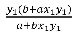
and 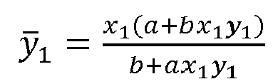
or the formula - P = (x̅ 1, y̅ 1) ∈ E with 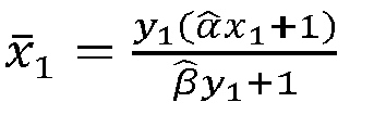
and 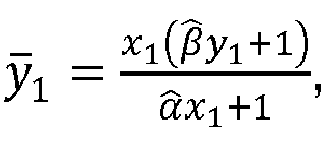
, where 
and 
calculating a point doubling using the formula [2]P = (x3, y3) with x3 = 
and 
calculating a point addition between the point P and a further finite point Q = (x 2, y 2) ∈ E, where P ≠ Q, using the formula P + Q = (x 3, y 3) with 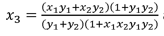
and 
and
calculating a point addition between the point P and a further finite point Q (x 2, y 2) ∈ E, where P may be equal to Q , using the formula P + Q = (x 3, y 3) with 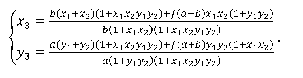
calculating a point inverse using the formula - P = (x̅ 1, y̅ 1) ∈ E with
calculating a point doubling using the formula [2]P = (x3, y3) with x3 =
calculating a point addition between the point P and a further finite point Q = (x 2, y 2) ∈ E, where P ≠ Q, using the formula P + Q = (x 3, y 3) with
calculating a point addition between the point P and a further finite point Q (x 2, y 2) ∈ E, where P may be equal to Q , using the formula P + Q = (x 3, y 3) with
Also provided is a processor (10).
Description
- The present invention relates generally to elliptic curves, and more particularly to unified addition formulae for Huff curves.
- This section is intended to introduce the reader to various aspects of art, which may be related to various aspects of the present invention that are described and/or claimed below. This discussion is believed to be helpful in providing the reader with background information to facilitate a better understanding of the various aspects of the present invention. Accordingly, it should be understood that these statements are to be read in this light, and not as admissions of prior art.
- Elliptic curve cryptography (ECC) is a technology of choice for the implementation of secure systems. A main advantage of it is the absence of sub-exponential algorithms to solve the underlying hard problem. Elliptic curve cryptosystems therefore feature smaller key sizes, which results in smaller memory and processor requirements and are thus especially well suited to memory-constrained devices such as smartcards.
- For the implementation of elliptic curve cryptosystems, two types of finite fields are mainly used: large prime fields and fields of characteristic 2. This description focuses on the binary case and only on non-supersingular elliptic curves, to prevent the so-called MOV reduction (see Alfred Menezes, Tatsuaki Okamoto, and Scott Vanstone. Reducing elliptic curve discrete logarithms to a finite field. IEEE Transactions on Information Theory, 39(5):1639-1646, 1993).
- An elliptic curve over a fieldis a smooth projective algebraic curve of genus 1 with a specified
 -rational point. More explicitly, when

 = (0 : 1 : 0). It is well known that the points on an elliptic curve given by a Weierstraß equation endows a group structure under the chord-and-tangent addition (see Joseph H. Silverman. The Arithmetic of Elliptic Curves, volume 106 of Graduate Texts in Mathematics, chapter III. Springer-Verlag, 1986). The identity element is
 . The inverse of a point P 0 = (x 0,y 0) ∈ E\{
 } is given by -P o = (x 0, y 0 + x 0). Hence, it appears that
 } and P 1 ≠ P 2, then


- There are other known models to represent elliptic curves (see e.g. David V. Chudnovsky and Gregory V. Chudnovsky. Sequences of numbers generated by addition in formal groups and new primality and factorization tests. Advances in Applied Mathematics, 7(4):385-434, 1986 and Explicit-formulas database (EFD), http://www.hyperelliptic.org/EFD/).
- Having different models at one's disposal is useful as this gives rise to a different arithmetic with different properties. An expected outcome is of course improved efficiency, which can be observed at different levels: speed, memory and processor requirements, bandwidth, etc. Another possible benefit is the ease of implementation. Of particular interest are the unified and complete addition laws, which reduce the number of cases to handle. The latter aspect can help preventing certain attacks, including those based on side-channel analysis (see Paul Kocher, Joshua Jaffe and Benjamin Jun. Differential power analysis. In M. Wiener, editor, Advances in Cryptology - CRYPTO '99, volume 1666 of Lecture Notes in Computer Science, pages 388-397. Springer-Verlag, 1999) or exceptional procedures (see Tetsuya Izu and Tsuyoshi Takagi. Exceptional procedure attack on elliptic curve cryptosystems. In Y.G. Desmedt, editor, Public Key Cryptography - PKC 2003, volume 2567 of Lecture Notes in Computer Science, pages 244-239. Springer, 2003). Yet another application resides in batch computing (see Daniel J. Bernstein. Batch binary Edwards. In S. Halevi, editor, Advances in Cryptology - CRYPTO 2009, volume 5667 of Lecture Notes in Computer Science, pages 317-336. Springer, 2009).
- A specific model for elliptic curves was introduced by Huff while studying a diophantine problem; see Gerald B. Huff. Diophantine Problems in Geometry and Elliptic Ternary Forms. Duke Math. J., 15:443-453, 1948; see also Williams D. Peeples, Jr. Elliptic Curves and Rational Distance Sets. Proc. Am. Math. Soc., 5:29-33, 1954.
- The Huff model was recently revisited by Marc Joye, Mehdi Tibouchi, and Damien Vergnaud in "Huff's Model for Elliptic Curves"; in G. Hanrot, F. Morain, and E. Thomé, editors, Algorithmic Number Theory (ANTS-IX), volume 6197 of Lecture Notes in Computer Science, pages 234-250, Springer , 2010. The paper fully covers fields of odd characteristic. For binary fields, an extended model is also proposed, but no details are given.
- A binary Huff curve is the set of projective points

 and a ≠ b.
- There are three points at infinity satisfying the curve equation: (a: b: 0), (1: 0: 0) and (0: 1: 0).
- The affine model corresponding to the binary Huff curve (Eq. (1)) is given by

- As stated in §3.4 of "Huff's Model for Elliptic Curves", this curve is birationally equivalent to the Weierstraß elliptic curve


- The set of points on a binary Huff curve forms a group whose identity element is o = (0,0). While these inverse maps are not line-preserving, the group law on a binary Huff curve satisfies the chord-and-tangent rule. lP,Q is the line joining points P and Q. This line intersects the curve in a third point (counting multiplicities) that is denoted by P*Q . l R,0 is the line through R := P*Q and o . The addition of P and Q is defined as the third point of intersection of l R,0 with the curve, that is, P + Q = R*o .
- However, the article in question provides no details, which means that the binary Huff curves may not be implemented. The present invention provides such details and can thus make it possible to use binary Huff curves for elliptic curve cryptography.
- In a first aspect, the invention is directed to a method for performing an arithmetic operation on a binary Huff curve defined by a set of projective points
 and a ≠ b. A processor obtains a first finite point P = (x 1, y 1) ∈ E, performs the arithmetic operation using the first point P to obtain a second point P' , and outputs the second point P' . The arithmetic operation comprises at least one of:
- calculating a point inverse using the formula -P = (
x 1,y 1) ∈ E withx 1 =

x 1 ,y 1 ) ∈ E with


- calculating a point doubling using the formula [2] P = (x 3, y 3) with x 3 =


- calculating a point addition between the point P and a further finite point Q = (x 2, y 2) ∈ E, where P ≠ Q , using the formula P + Q = (x 3, y 3) with x 3 =


- calculating a point addition between the point P and a further finite point Q = (x 2, y 2) ∈ E, where P may be equal to Q , using the formula P + Q = (x 3, y 3) with

- In a first preferred embodiment, = 1.
- In a second preferred embodiment, the method is a cryptographic method.
- In a second preferred embodiment, the method further comprises a preceding step of transforming a point on a first elliptic curve v(v + (a + b) fu) = u(u + a 2)(u + b 2) into the first point P on the binary Huff curve under the map


- In a second aspect, the invention is directed to a processor for performing an arithmetic operation on a binary Huff curve defined by a set of projective points
 and a ≠ b. The processor is adapted to obtain a first finite point P = (x 1,y 1) ∈ E, perform the arithmetic operation using the first point P to obtain a second point P' , and output the second point P' . The arithmetic operation comprises at least one of:
- calculating a point inverse using the formula -P = (
x 1,y 1) ∈ E withx 1 =

x 1,y 1) ∈ E with


- calculating a point doubling using the formula [2] P = (x 3,y 3) with x 3 =


- calculating a point addition between the point P and a further finite point Q = (x 2,y 2) ∈ E, where P ≠ Q , using the formula P + Q = (x 3,y 3) with x 3 =


- calculating a point addition between the point P and a further finite point Q = (x 2,y 2) ∈ E, where P may be equal to Q , using the formula P + Q = (x 3,y 3) with

- Preferred features of the present invention will now be described, by way of non-limiting example, with reference to the accompanying drawings, in which
-
Figure 1 illustrates a device for performing cryptography calculations according to a preferred embodiment of the present invention. - The description now provides details about the binary Huff curves introduced in the background section of the present application.
- Point inverse Identity element o is not an inflection point. The inverse of a point P is therefore not defined as P*o . -P = P *A , where

- Another way to get the inverse is to use the birational equivalence with the Weierstraß form. P = (x 1,y 1) ∈ E is a finite point. Then, whenever defined, -P = (
x 1,y 1) ∈ E with


For the points at infinity, -(a: b: 0) = (a: b: 0), -(1:0:0) =

- Point doubling The birational equivalence could also be used to derive the doubling formula, but, as the calculation is difficult, it is easier to rely on the geometric interpretation of the addition law.
- P = (x 1,y 1) ∈ E is a finite point. The third point of intersection of the tangent line to the curve at P is S = P * P . Then [2] P = S * o , which gives [2] P = (x3 ,y 3) with

- It should be noted that since a solution to ζ2 + ζ + 1 = 0 is a non-trivial cubic root of unity, (ζ,ζ-1) is a rational point if and only if the curve is defined over a binary extension field of even degree (i.e. overwith n even). It should also be noted that (ζ,ζ-1) has order 4.

For the points at infinity, [2] (a: b: 0) = o (since (a: b: 0) has order 2), and [2] (1: 0: 0) = [2] (0: 1: 0) = A , where
- P = (x 1,y 1) and Q = (x 2,y 2) ∈ E are two finite points with P # Q . As already mentioned, the addition of P and Q is given by P + Q = ( P * Q )* o. Then, whenever defined, P + Q = (x 3,y 3) with

- It should be noticed that when x 1 = x 2, it may be assumed that y 1 ≠ 0; otherwise x 1 = x 2 = 0 and thus P = Q = o . Then (x 1,y 1) +


- Supposing that x 1 ≠ x 2 and y 1 ≠ y 2, if x 1 x 2 y 1 y 2 = 1 and x 1 x 2 = 1, then P + Q = [2] P + (a: b: 0). If x 1 x 2 y 1 y 2 = 1 and x1x2 ≠ 1, then P + Q = (a: b: 0).
- When P = (x 1,y 1) is finite and Q is at infinity, then


- In addition, (a:b:0) + (1 :0:0) = (0:1:0), (a:b:0) + (0:1 :0) = (1:0:0), and (1:0:0) + (0:1:0)=

- Projective formulae The addition formulae may also be expressed in a projective version. The doubling (Eq. (4)) of P = (X 1 : Y 1 : Z 1) may be expressed as


- For more efficient computation, this may be evaluated as


- The dedicated addition (Eq. (5)) of P = (X 1 : Y 1 : Z 1) and Q = (X 2 : Y 2 : Z 2) may be expressed as


- For more efficient computation, this may be evaluated as


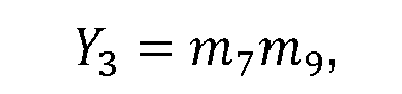

- Even more efficient computation evaluates this, with extended coordinates (X i, Y i, Z i, T i) where T i = X i Y i (i = 1,2,3), as


- The formulae for evaluation of P + Q hereinbefore distinguish between doubling ( P = Q ) and dedicated addition (P ≠ Q), as the dedicated addition formula is undefined when P = Q . It would therefore be desirable to have a unified point addition operation that can be used in both cases.
- Equation (5), i.e. the formula for dedicated point addition states that with P = (x 1,y 1) and Q = (x 2,y 2) ∈ E being two finite points with P ≠ Q , then whenever defined, P + Q = (x 3,y 3) with

- The point addition is defined up to the curve equation. Using the additional relations axi (yi 2 + yi + 1) = byi (xi 2 + xi + 1), i ∈ {1,2} gives

- Remarkably, these new expressions also work for doubling a point P = (x 1,y 1). Indeed, setting (x 2,y 2) = (x 1,y 1) in Equation (6) gives (since the binary characteristic entails that two times any value equals zero)

- This may be compared with Equation (4)

- Given that (1+A)2 = (1+A 2) because of the binary characteristic, it may easily be seen that the expressions are equal.
- The unified addition law given by Equation (6) is defined when the denominators b(1 + x 1 x 2 )(1 + x 1 x 2 y 1 y 2) and a(1 + y 1 y 2)(1 + x 1 x 2 y 1 y 2) are non-zero. If x 1 x 2 y 1 y 2 = 1, x 1 x 2 ≠ 1 and y 1 y 2 ≠ 1, then P + Q = (a : b : 0). If x 1 x 2 = 1 or y 1 y 2 = 1, i.e. P = (x 1,y 1) (≠ o ) and Q ∈


- The cases where the points P , or Q , or P and Q , are at infinity have already been discussed hereinbefore.
- Since the case P = (x 1, y 1) and Q ∈
 and
and

- In particular, the addition formula is complete in a subgroup of odd order, provided that both (1 : 0 : 0) and (0 : 1 : 0) are of even order.
- Projective version The unified addition (Equation (6)) P + Q = (X3 : Y 3 : Z 3 ), where P = (X 1 : Y 1 : Z 1) and Q = (X 2 : Y 2 : Z 2), may be expressed as


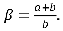
- For more efficient computation, this may be evaluated as



- More formulae There are, naturally, other unified addition formulae that are similar to Equation (6). For instance, whenever defined

- In general, alternate unified formulae may be obtained by selecting another neutral element. This results in translating the group law. For instance, defining o' = (a : b : 0) as the neutral element yields, whenever defined, the following unified point addition formula

- The corresponding projective version can advantageously be evaluated as


- In order to speed up the implementation of the elliptic curve factoring method (ECM) (see Hendrik W. Lenstra, Jr. Factoring Integers with Elliptic Curves. Annals of Mathematics, 126(2): 649-673, 1987) the so-called Montgomery representation was developed (see Peter L. Montgomery. Speeding up the Pollard and Elliptic Curve Methods of Factorization. Mathematics of Computation, 48(177):243-264; 1987). It was subsequently adapted to (ordinary) Weierstraß elliptic curves over binary fields (see Julio López and Ricardo Dahab. Fast Multiplication on Elliptic Curves over GF(2m) without Precomputation. In Ç. Koç and C. Paar, editors, Cryptographic Hardware and Embedded Systems - CHES '99, volume 1717 of Lecture Notes in Computer Science, pages 316-327. Springer, 1999 - see also Martijn Stam. On Montgomery-like Representations for Elliptic Curves over GF(2k). In Y.G. Desmedt, editor, Public Key Cryptography - PKC 2003, volume 2567 of Lecture Notes in Computer Science, pages 240-253. Springer, 2003 - and also Pierrick Gaudry and David Lubicz. The Arithmetic of Characteristic 2 Kummer Surfaces and of Elliptic Kummer Lines. Finite Fields and Applications, 15:246-260, 2009).
- The idea stems from the observation that the x-coordinate of the sum of two points can be evaluated from the x-coordinates of the input points and the x-coordinate of their difference.
- More generally, a differential point addition comprises calculating w(P + Q) from w(P), w(Q) and w(P - Q) for a certain coordinate function w. When such an operation is available, the value of w([k]P) can be efficiently computed from the binary expansion of scalar k,



- As already shown hereinbefore, the inverse of a point P = (x1, y1) on a binary Huff curve is given by -P = (x̅ 1, y̅ 1) with


- Specifically, for a finite point P = (x1, y1) is defined w( P ) = x 1 y 1. For the points at infinity, the following is defined:


- Q is a second point, different from P , and w 1, w 2 and w̅ respectively denote the w-coordinates of P , Q and Q-P. It could in principle be possible to derive the formula for the differential addition from Equation (5), but a much simpler way is to rely on the connection between the choice of the w-coordinate and the birational map with the Weierstraß equation; cf. Equation (2).
- Montgomery representation comes in two flavours: additive method and multiplicative method. The additive formula (Lemma 1 provided by López and Dahab, slightly generalized), whenever defined, gives

- An application of the multiplicative formula (§ 3.2) provided by Martijn Stam yields after simplification

- To obtain projective formulae, the w-coordinate of a point P is represented by the pair (W : Z) = (Θw(P) : Θ) if P ≠ (a : b : 0), and (W : Z) = (Θ : 0) if P = (a : b : 0), for some non-zero Θ∈F2m. Letting w i = (Wi : Zi ) for i = 1, 2, and w̅ = (W̅ : Z̅), Equations (8) and (9) give

- The transformations given by Equation (2) show how to express any binary Huff curve as a Weierstraß curve. The reverse is however not always possible: not all ordinary elliptic curves over F2m can be expressed in the Huff form of Equation (1). Worse, none of the curves recommended by NIST (see National Institute of Standards and Technology. Recommended elliptic curves for federal government use. http://csrc.nist.gov/CryptoToolkit/dss/ecdsa/NISTeCur.pdf, July 1999) can be written in this model. The definition of binary Huff curves is therefore generalized hereinafter to cover all isomorphism classes of ordinary curves over F2m for m ≥ 4.
- In section 3 of "Huff's Model for Elliptic Curves", Huff's model is generalized to axP(y) = byP(x) for some monic polynomial P ∈ F 2 m[t], of degree 2, with non-zero discriminant, and such that P(0) ≠ 0. Binary Huff curves correspond to the choice P (t) = t2 + t + 1. A more general polynomial, namely P (t) = t2 + ft + 1 with f ≠ 0, is considered hereinafter.
- The following definition is then possible: a generalized binary Huff curve is the set of projective points (X : Y : Z) ≥ P2 (F2m) satisfying the equation

- There are naturally other suitable generalizations of binary Huff curves, such as P (t) = t 2 + t + e with e ≠ 0. It should be noted that the polynomial P (t) = t 2 + ft + e with e,f ≠ 0 is not more general as a change of variables can transform this equation into one of the other possible forms.
- The affine model of
Equation 10 is ax(y 2 + fy + 1) = by(x2 + fx + 1), which is birationally equivalent to the Weierstraß elliptic curve

- The points at infinity are (a : b : 0), (1 : 0 : 0) and (0 : 1 : 0). Point A , i.e. the point of intersection of the tangent line at o with the curve, becomes

- Thus, for m ≥ 4, each ordinary elliptic curve over F2 m is birationally equivalent over F2 m to a generalized binary Huff curve.
- It is then possible - and it may be of interest for reasons of performance and security - to transform an elliptic curve over F2 m into a generalized binary Huff curve. Then the formulae given hereinafter may be used for calculations and the result may be transformed back to the original elliptic curve.
- The arithmetic on generalized binary Huff curves is easily derived from the formulae given hereinbefore. Et is a generalized binary Huff curve as per Equation (10) and P = (x 1, y 1) and Q = (x 2, y 2) ∈ E + are two finite points. The formula given by Equation (3) remains valid for computing the inverse of P . An alternate expression for - P is, whenever defined,


- The doubling formula (Equation (4)) becomes [2] P = (x 3, y 3) with

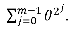
- The formula for dedicated point addition (Equation (5)) remains unchanged.
- The formula for unified point addition is, whenever defined, P + Q = (x 3,y 3) with

- Equation (6') becomes:

- The formula for changing the neutral element (6") is:
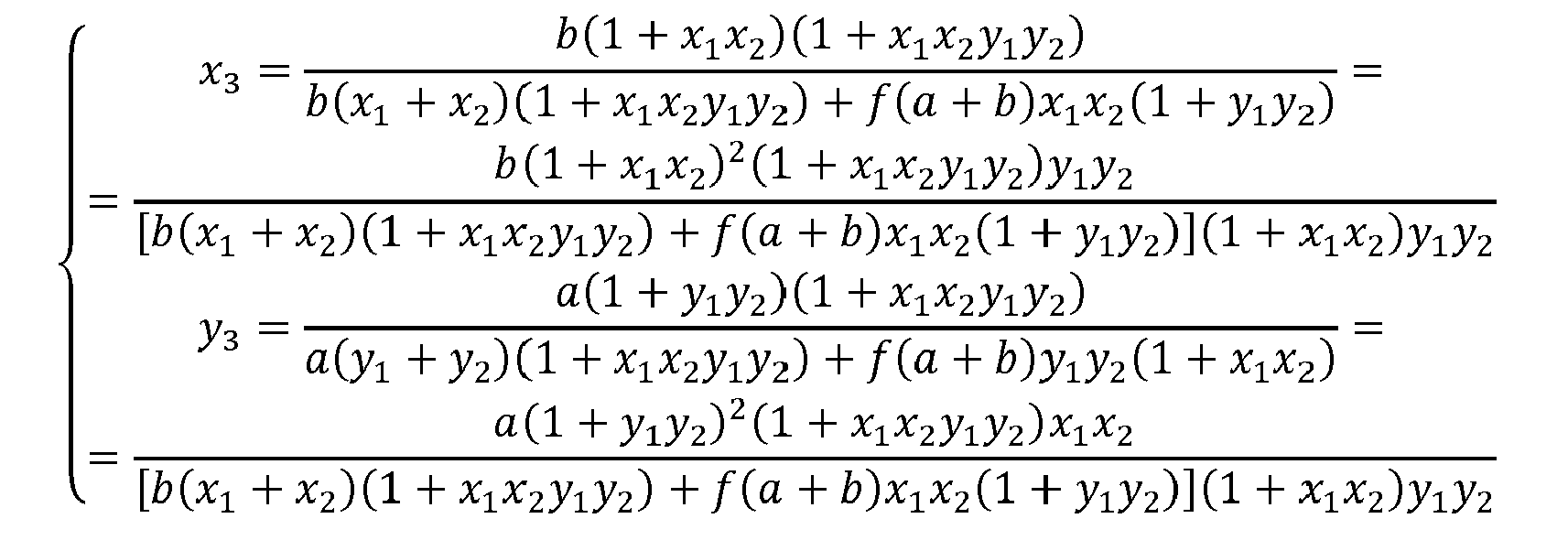
- The evaluation of the corresponding projective formula except that


-
Figure 1 illustrates adevice 10 for performing elliptic curve cryptography calculations using the binary Huff curves described herein. Thedevice 10 is preferably a processor, advantageously a secure cryptoprocessor, which receives input that is processed and then output. - Elliptic curve cryptography uses point multiplication to arrive at an output. Indeed, as mentioned on Wikipedia (Elliptic curve cryptography): "The entire security of ECC depends on the ability to compute a point multiplication and the inability to compute the multiplicand given the original and product points."
- Generally speaking, the prior art (see "Elliptic curve cryptography" on Wikipedia) has provided different ways performing point multiplication, for example repeated point addition and double-and-add of which the latter has sprouted efficient variants such as the "windowed method", the "sliding-window method" and the "Montgomery ladder".
- During elliptic curve cryptography calculations, the
processor 10 receives a point as input, performs at least one point multiplication using the point and outputs the result. - An example of practical use is the Diffie-Hellman key exchange. Alice and Bob have agreed on an elliptic curve and a point P on the curve, both of which may be public. Alice chooses a secret integer ka and Bob independently chooses a secret integer kb . Alice sends [k a] P to Bob and receives [k b] P in return. Then Alice and Bob calculated the common secret key as [kakb ] P, which naturally also is a point on the curve.
- The multiplicand may for example also be a secret key. It will be appreciated that the point P and the multiplicand may be received as input to the processor, but it is also possible for one or the other, or both, to be stored in the processor itself, for example as part of a program being executed.
- Each feature disclosed in the description and (where appropriate) the claims and drawings may be provided independently or in any appropriate combination. Reference numerals appearing in the claims are by way of illustration only and shall have no limiting effect on the scope of the claims.
Claims (5)
- A method for performing an arithmetic operation on a binary Huff curve defined by a set of projective points (X : Y : Z) ∈ P2(F 2 m) satisfying the equation aX(Y 2 + fYZ + Z 2) = bY (X 2 + fXZ + Z 2), where a, b, f ∈ F*2 m and a ≠ b, the method comprising the steps, performed by a processor (10), of:- obtaining a first finite point P = (x 1, y 1) ∈ E,- performing the arithmetic operation using the first point P to obtain a second point P ', and- outputting the second point P ',wherein the arithmetic operation comprises at least one of:calculating a point inverse using the formula


 calculating a point doubling using the formula [2] P = (x3, y3 ) with

 calculating a point addition between the point P and a further finite point Q = (x2,y2) ∈ E, where P may be equal to Q , using the formula P + Q = (x 3,y 3) with
- The method of claim 1, wherein f = 1.
- The method of claim 1, the method is a cryptographic method.
- The method of claim 1, further comprising:- a preceding step of transforming a point on a first elliptic curve v(v + (a + b) fu) = u(u + a 2)(u + b 2) into the first point P on the binary Huff curve under the mapwherein the step of performing the arithmetic operation comprises obtaining an intermediate point P " on the binary Huff curve that is transformed into the second point P' on the first elliptic curve under the map


- A processor (10) for performing an arithmetic operation on a binary Huff curve defined by a set of projective points (X : Y : Z) ∈ P2(F2 m) satisfying the equation aX(Y2 + fYZ + Z2) = bY(X2 + fXZ + Z 2), where a, b, f ∈ F*2 m and a ≠ b, the processor (10) being adapted to:- obtain a first finite point P = (x1,y1) ∈ E,- perform the arithmetic operation using the first point P to obtain a second point P ', and- output the second point P ',wherein the arithmetic operation comprises at least one of:calculating a point inverse using the formula - P = (x̅1, y̅ 1) ∈ E with


 calculating a point doubling using the formula [2] P = (x 3, y 3) with

 calculating a point addition between the point P and a further finite point Q = (x2,y2) ∈ E, where P ≠ Q, using the formula P + Q = (x 3, y 3) with

 calculating a point addition between the point P and a further finite point Q = (x 2,y 2 ) ∈ E, where P may be equal to Q , using the formula P + Q = (x 3, y 3) with
Priority Applications (1)
| Application Number | Priority Date | Filing Date | Title |
|---|---|---|---|
| EP10306285A EP2421193A1 (en) | 2010-08-20 | 2010-11-23 | Method and processor for performing arithmetic operations on binary Huff curves |
Applications Claiming Priority (2)
| Application Number | Priority Date | Filing Date | Title |
|---|---|---|---|
| EP10290452 | 2010-08-20 | ||
| EP10306285A EP2421193A1 (en) | 2010-08-20 | 2010-11-23 | Method and processor for performing arithmetic operations on binary Huff curves |
Publications (1)
| Publication Number | Publication Date |
|---|---|
| EP2421193A1 true EP2421193A1 (en) | 2012-02-22 |
Family
ID=45002199
Family Applications (1)
| Application Number | Title | Priority Date | Filing Date |
|---|---|---|---|
| EP10306285A Withdrawn EP2421193A1 (en) | 2010-08-20 | 2010-11-23 | Method and processor for performing arithmetic operations on binary Huff curves |
Country Status (1)
| Country | Link |
|---|---|
| EP (1) | EP2421193A1 (en) |
-
2010
- 2010-11-23 EP EP10306285A patent/EP2421193A1/en not_active Withdrawn
Non-Patent Citations (17)
Similar Documents
| Publication | Publication Date | Title |
|---|---|---|
| Joye et al. | Hessian elliptic curves and side-channel attacks | |
| Billet et al. | The Jacobi model of an elliptic curve and side-channel analysis | |
| López et al. | Fast multiplication on elliptic curves over GF (2m) without precomputation | |
| Wiener et al. | Faster attacks on elliptic curve cryptosystems | |
| KR101154695B1 (en) | Encryption computing device | |
| Devigne et al. | Binary huff curves | |
| Rondepierre | Revisiting atomic patterns for scalar multiplications on elliptic curves | |
| Satoh | Generating genus two hyperelliptic curves over large characteristic finite fields | |
| Subramanya Rao | Three dimensional Montgomery ladder, differential point tripling on Montgomery curves and point quintupling on Weierstrass’ and Edwards curves | |
| Ajeena et al. | Comparison Studies on Integer Decomposition Method for Elliptic Scalar Multiplication | |
| Lee et al. | Parallelized Scalar Multiplication on Elliptic Curves Defined over Optimal Extension Field. | |
| da Silva et al. | Isogeny formulas for Jacobi intersection and twisted hessian curves. | |
| Dang et al. | Twisted hessian isogenies | |
| Dryło et al. | Determining formulas related to point compression on alternative models of elliptic curves | |
| JP4599859B2 (en) | Cryptographic processing operation method, cryptographic processing apparatus, and computer program | |
| Guo et al. | Efficient scalar multiplication of ECC using SMBR and fast septuple formula for IoT | |
| Gajbhiye et al. | A survey report on elliptic curve cryptography | |
| US20040001590A1 (en) | Efficient elliptic curve double-and-add calculator | |
| Takashima | A new type of fast endomorphisms on Jacobians of hyperelliptic curves and their cryptographic application | |
| Le et al. | Fast point quadrupling on elliptic curves | |
| Schoof | The discrete logarithm problem | |
| Duquesne | Traces of the group law on the Kummer surface of a curve of genus 2 in characteristic 2 | |
| Ciss et al. | On a new generalization of Huff curves | |
| EP2085878A1 (en) | An apparatus and a method for calculating a multiple of a point on an elliptic curve | |
| Egrice et al. | p261: A Karatsuba-Friendly Prime for Fast Elliptic Curve Arithmetic |
Legal Events
| Date | Code | Title | Description |
|---|---|---|---|
| AK | Designated contracting states |
Kind code of ref document: A1 Designated state(s): AL AT BE BG CH CY CZ DE DK EE ES FI FR GB GR HR HU IE IS IT LI LT LU LV MC MK MT NL NO PL PT RO RS SE SI SK SM TR |
|
| AX | Request for extension of the european patent |
Extension state: BA ME |
|
| PUAI | Public reference made under article 153(3) epc to a published international application that has entered the european phase |
Free format text: ORIGINAL CODE: 0009012 |
|
| STAA | Information on the status of an ep patent application or granted ep patent |
Free format text: STATUS: THE APPLICATION IS DEEMED TO BE WITHDRAWN |
|
| 18D | Application deemed to be withdrawn |
Effective date: 20120823 |