EP2309289A1 - Method for separating interleaved radar pulses sequences - Google Patents
Method for separating interleaved radar pulses sequences Download PDFInfo
- Publication number
- EP2309289A1 EP2309289A1 EP10176487A EP10176487A EP2309289A1 EP 2309289 A1 EP2309289 A1 EP 2309289A1 EP 10176487 A EP10176487 A EP 10176487A EP 10176487 A EP10176487 A EP 10176487A EP 2309289 A1 EP2309289 A1 EP 2309289A1
- Authority
- EP
- European Patent Office
- Prior art keywords
- pulses
- dtoa
- pulse
- pri
- search range
- Prior art date
- Legal status (The legal status is an assumption and is not a legal conclusion. Google has not performed a legal analysis and makes no representation as to the accuracy of the status listed.)
- Granted
Links
- 238000000034 method Methods 0.000 title claims abstract description 23
- 238000005070 sampling Methods 0.000 claims description 18
- 238000004364 calculation method Methods 0.000 claims description 14
- 238000000926 separation method Methods 0.000 claims description 7
- 238000005259 measurement Methods 0.000 claims description 3
- 238000013139 quantization Methods 0.000 claims description 2
- 239000000428 dust Substances 0.000 claims 1
- 230000009466 transformation Effects 0.000 abstract description 3
- 239000011295 pitch Substances 0.000 description 8
- 239000012141 concentrate Substances 0.000 description 2
- 101710131167 Ribose-5-phosphate isomerase A 2 Proteins 0.000 description 1
- 230000005540 biological transmission Effects 0.000 description 1
- 238000010276 construction Methods 0.000 description 1
- 238000001514 detection method Methods 0.000 description 1
- 238000005286 illumination Methods 0.000 description 1
- 239000000203 mixture Substances 0.000 description 1
Images


Classifications
-
- G—PHYSICS
- G01—MEASURING; TESTING
- G01S—RADIO DIRECTION-FINDING; RADIO NAVIGATION; DETERMINING DISTANCE OR VELOCITY BY USE OF RADIO WAVES; LOCATING OR PRESENCE-DETECTING BY USE OF THE REFLECTION OR RERADIATION OF RADIO WAVES; ANALOGOUS ARRANGEMENTS USING OTHER WAVES
- G01S7/00—Details of systems according to groups G01S13/00, G01S15/00, G01S17/00
- G01S7/02—Details of systems according to groups G01S13/00, G01S15/00, G01S17/00 of systems according to group G01S13/00
- G01S7/021—Auxiliary means for detecting or identifying radar signals or the like, e.g. radar jamming signals
Definitions
- the invention relates to a method for separating nested radar pulse trains. It applies in particular in the presence of several pulse trains whose pulse repetition periods are close or when the repetition period of the pulses of a train fluctuates randomly or pseudo-random around a mean value.
- the devices whose function is to monitor the emissions of radars, require the ability to separate and characterize each transmission in the total flow corresponding to all the present emissions received, and in particular when these are locally nested, it is i.e., nested within a short period of time substantially corresponding to all or part of an illumination duration.
- a first technique for separating a pulse train belonging to a given radar, the complete flow of all pulses received, is based on the construction of histograms of arrival time differences, or Difference of Time of Arrival (DTOA) according to the Anglo-Saxon expression, successive impulses.
- DTOA Difference of Time of Arrival
- This technique works well in the presence of radar signals whose pulse repetition periods (PRIs) are relatively spaced from each other and remain constant.
- this technique is not robust to the fluctuations of the PRI, especially in the presence of several locally nested radar signals whose average PRIs are relatively close.
- the distribution of the fluctuations can not be described by the histogram continuously. It is then difficult to determine a mean PRI.
- a second technique is based on the use of the discrete Fourier transform applied at the time of arrival, or Time Of Arrival (TOA) according to the Anglo-Saxon expression, impulses.
- TOA Time Of Arrival
- the Fourier transform makes it possible to concentrate the DTOAs of the same pulse train towards its average PRI and to separate pulse trains from several locally nested radars.
- the Fourier transform also has the advantage of being only slightly impeded by missing pulses.
- the sampling step of the calculation frequencies must be relatively small in order to calculate the Fourier transform at a frequency close to the pulse repetition frequency (FRI) or, if appropriate, the average FRI. Consequently, since the calculation cost of the Fourier transform is proportional to the product of the number of pulses by the number of calculation frequencies, it is generally important and prevents a so-called real-time processing of the radar signals.
- FRI pulse repetition frequency
- the search range ⁇ t c is defined by the lower bound of the first class containing a number of pulses greater than or equal to a predetermined threshold, and by the upper bound of the last class containing a number of pulses. impulses greater than or equal to the predetermined threshold.
- the classes of the histogram of DTOA may have the same range width, this width then defines a histogram step p h , the histogram step p h being determined to be of the order of 30 to 50 times the measurement and quantization error of the arrival times TOA k pulses.
- DFT discrete Fourier transform
- the invention has the particular advantage that it allows to use the separating power of the Fourier transform without requiring a significant calculation cost.
- the radar signal comprises N radar pulses received and dated at their arrival during an acquisition period D.
- the radar pulses are for example received and dated by a receiver of measurements.
- Each radar pulse thus gives rise to a arrival time TOA k , with k being between 1 and N.
- the pulses can come from a single transmitter or from several transmitters, each transmitter providing a pulse train whose repetition period pulses (PRI) is likely to fluctuate around an average PRI.
- a pulse train whose PRI fluctuates is called a PRI train.
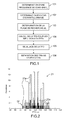
- the figure 1 represents possible steps for the method of separating pulse trains according to the invention.
- a first step 101 one or more reference frequencies f c are determined around which a discrete Fourier transform (DFT) will be calculated.
- a sampling step ⁇ f for the DFT is determined.
- a search range ⁇ f c is determined on which the DFT will be calculated.
- a DFT for the TOA k is calculated as a function of the search range ⁇ f c and the sampling pitch ⁇ f determined previously.
- the DFT is thresholded.
- the thresholded DFT is used to determine the FRI of the pulse trains. present and separate them.
- the method of separating pulse trains according to the invention is based on the calculation of the discrete Fourier transform (DFT) applied to the arrival times TOA k pulses.
- DFT discrete Fourier transform
- FRI pulse repetition frequency or frequencies
- the DFT can be calculated only around this or these FRI. Operation is for example supervised when a pulse train has previously been detected and characterized, and there is a good chance that it will reappear with the same FRI. Beyond this supervision context, it is sought to determine a range of frequencies in which FRI are likely to be identified. This frequency range is called the search range ⁇ f c . It is for example centered on a set frequency f c .
- the set frequency f c is determined in a first step 101 from an arrival time difference (DTOA) histogram.
- Histograms of DTOA can be constructed for different orders. The order of the order depends on the context of use of the invention.
- a DTOA histogram of given order m is constructed by determining, for each pulse arriving at time TOA k , the time separating it from the pulse arriving at the moment TOA km , that is to say its DTOA. of order m, and grouping neighboring DTOA pulses within classes, each class being defined by a range of DTOA and a number of pulses. All classes can have the same range width. The range width then defines a histogram step p h .
- the pitch p h is chosen to be wide enough to detect a PRI pulse train that is jittered on a small number of adjacent classes. Indeed, if the histogram step p h is too fine, the DTOA may be spread over many non-adjacent classes. It is then difficult to differentiate the relevant classes, that is to say those containing DTOA actually corresponding to a PRI value, classes formed by the noise, for example due to missing pulses. Conversely, the histogram not ph does not should not be too large to avoid grouping of all pulses in one class. According to a particular embodiment, the histogram step p h is determined to be of the order of 30 to 50 times this error for the detection of jittered PRI pulse trains.
- the search range ⁇ f c for the calculation of the DFT can thus be determined from the classes of the histogram.
- a search range ⁇ t c in the time domain (DTOA) defined by the lower bound of the first class containing at least one pulse and by the upper bound of the last class containing at least one pulse.
- the average DTOA of the search range ⁇ t c is called DTOA of setpoint DTOA c .
- the average considered is for example the arithmetic mean.
- the set frequency f c is then defined by the inverse of this set DTOA DTOA c .
- the DFT is calculated around this frequency f c over the search range ⁇ f c .
- the search range ⁇ t c is then bounded by a minimum DTOA corresponding to the lower bound of the first class containing a number of pulses greater than or equal to the threshold and by a maximum DTOA corresponding to the upper bound of the last class containing a number pulses greater than or equal to the threshold. Classes containing a number of pulses below the threshold may be considered as containing no pulse.
- two distinct search ranges ⁇ t are considered. c1 and ⁇ t c2 .
- the figure 2 illustrates the influence of pitch on the shape of the DTOA histogram.
- Two histograms are shown for the same train of 100 pulses with an average MIC of 100 microseconds ( ⁇ s) clocked by 30% ( ⁇ 15% from the central value).
- the first histogram 21 is constructed with a pitch of 3 ⁇ s and the second histogram 22 is constructed with a pitch of 0.3 ⁇ s.
- the classes of the first histogram 21 are denoted 21a and the classes of the second histogram are denoted 22a.
- the DTOA setpoint DTOA c would be determined around 100 ⁇ s and the search range ⁇ t c would be between approximately 88 ⁇ s and 118 ⁇ s, ie a range of 30 ⁇ s.
- the reference frequency f c Since the reference frequency f c has been determined, it remains in particular to determine the sampling step ⁇ f of the calculation frequencies for the discrete Fourier transform.
- the determination of the sampling step ⁇ f is the subject of step 102.
- the DFT calculated on the TOA k pulses has a lobe width around the Average FRI at least equal to 2 / D. Indeed, when the first and the last pulse belong to the same pulse train, the effective duration of the pulse train is equal to D. The width of the main lobe of the DFT is then equal to 2 / D.
- the effective duration of one of the pulse trains may be lower and therefore the main lobe of its DFT may be wider than 2 / D.
- the train T1 is only present part of D and therefore the lobe of the TF relative to its PRI will have a width of 4 / D, much wider than that which one could expect.
- the frequency range ⁇ f c can also be expressed in percentage P of the set DTOA DTOA c .
- the resolution in PRI ⁇ pri is not.
- the field of application of the DFT can be limited according to the number N min of pulses in the radar signal.
- the DFT should not normally be calculated for frequencies corresponding to PRI greater than D / N min .
- a jitter rate of a PRI of ⁇ J / 2% with a DFT it is necessary to have at least 100 / J pulses. By way of example, it takes at least 10 pulses to correctly estimate, with the DFT, a PRI jittered by plus or minus 5%, or it takes at least 20 pulses for a PRI jittered by plus or minus 2.5%.
- a fourth step 104 the discrete Fourier transform S (f) of the radar signal s (t) is calculated for the arrival times TOA k of the pulses.
- the figure 3 illustrates the effect of the DFT on a pulse train whose PRI is released.
- the train has 100 pulses with an average PRI of 100 ⁇ s jitter by 10% ( ⁇ 5% of the central value).
- On the figure 3 is shown a histogram of DTOA 41 built for this pulse train with a pitch of 1 ⁇ s. The histogram shows a large spreading making it difficult to determine the average PRI of the train.
- the DFT of the radar signal is also represented graphically on the figure 3 by its components 42 and by an interpolation of its components 43.
- the sampling rate in frequency chosen for the DFT is 1 / D.
- the DFT concentrates its energy around the average PRI and allows to estimate it with a resolution of 1 / D.
- This concentration of energy is visible on the figure 3 by the presence of a main peak 44 around 100 ⁇ s.
- the higher amplitude component 42 can be considered as the average FRI.
- the higher amplitude component corresponds to a PRI of about 100.2 ⁇ s.
- the average FRI of the pulse train is therefore approximately equal to 9.98 kHz.
- the higher amplitude component 42 does not necessarily correspond to the maximum of the non-sampled Fourier transform. But even a very small difference in the average FRI estimate can be troublesome for the rest of the process. In order to reduce this error, it is possible to interpolate the DFT around its component 42 of greater amplitude.
- the DFT can for example be interpolated by a simple parabolic expression because of the virtually parabolic shape of the main peak.
- the figure 4 represents the interpolation of the DFT around its component 42 of greater amplitude by a parabola.
- the reference frequency f c , the components 42 of the DFT, the non-sampled Fourier transform 51 and a parabola 52 interpolating the DFT are plotted on the figure 4 according to of the frequency.
- the parabola 52 is constructed from the component 42 of greater amplitude and its two adjacent components 42.
- the figure 5 illustrates, according to a representation similar to that of the figure 3 , the effect of the DFT on two pulse trains whose PRI are set at 10% ( ⁇ 5% of the central value). Each train has 50 pulses. The first train has an average PRI of 100 ⁇ s and the second train has an average PRI of 102 ⁇ s. A histogram of DTOA 61 with a pitch of 1 ⁇ s is constructed for both pulse trains. The figure 5 shows that it is impossible to determine the average PRI from the histogram 61. This figure is also represented graphically the DFT applied to the two pulse trains, by its components 62 and by an interpolation of its components 63. No frequency sampling chosen for the DFT is also 1 / D.
- the DFT has two main peaks 64 and 65 centered on the average PRIs of the two pulse trains. It is then possible to determine these average PRI from the components 62 of greater amplitude. Consequently, in the presence of several pulse trains whose average PRIs are close, the concentration power of the DFT also implies a separation power of the PRIs.
- the figure 6 illustrates the influence of the rate of fluctuation of the PRI (jitter) on the module of the DFT at its main peak.
- the gain G is plotted against the jitter rate in percent.
- the figure 6 shows that even with a jitter rate of 30% ( ⁇ 15% of the central value), the module loses only 15% of the value it would have in the absence of jitter.
- jitter has a relatively weak influence on the shape of the main peak. It does not affect the resolution of the DFT, which only depends on the acquisition time D of the radar signal.
- the maximum of the DFT can be compared to a s threshold DFT in a fifth step 105.
- a train of repetition frequency of pulses of the pulse f RI observed over a period D gives a number of pulses equal to the product RI Df.
- the product Df RI can be weighted by a weighting coefficient.
- mitage means the lack of one or more pulses in a pulse train, for example due to the non-receipt of this or these pulses.
- the rate of mourning is the percentage of missing pulses of a train compared to the total number of pulses of this train. For example, for a maximum allowable jitter rate J max of 40%, corresponding to a G gain of 0.75, and a maximum permissible mite rate Tm max of 60%, the weighting coefficient is equal to 0 3.
- N min is an operational setting. It is for example equal to five.
- S TFD max ⁇ BOY WUT J max . 1 - tm max . D . f Services , NOT min .
- the histogram of DTOA built in step 101 has disjoint classes or not. If the PRIs of the trains are sufficiently different from each other, the classes of the histogram form groups of disjoint classes. The pulses of each train can then be separated according to the class group to which they belong. It is then not necessary to calculate the DFT on the TOA k of these pulses. On the other hand, if the PRIs of the different trains fluctuate and are close, the classes of the histogram form only one group thus offering no more resolution. The DFT can then be calculated on the TOA k pulses according to step 104.
- the DFT allows two disjoint peaks to be observed when the difference of PRI is large enough in relation to its separating power. Its different main peaks make it possible to precisely determine the average PRI of each pulse train. This knowledge then makes it possible, in a step 106, to separate the pulses relative to the train to which they belong.
- the separation of the pulse trains is performed by analyzing the phase of the pulses.
- the phase may not be quite constant due to the fluctuation of the PRI. However, the phase evolves in this case around an average value.
- the figure 7 represents the evolution of the pulse phase of a radar signal as a function of their arrival time TOA k for two different PRIs.
- a first graph 81 is plotted for a PRI of 100 ⁇ s, ie for the average PRI determined after Fourier transform for a first pulse train, and the graph 82 is plotted for a PRI of 110 ⁇ s, ie for the determined average PRI. after Fourier transformation for a second pulse train.
- the graph 81 makes it possible to highlight the presence in the radar signal of the first pulse train 83 with an average PRI of 100 ⁇ s and to separate the pulses of this first train. It also highlights the presence of one or more other trains 84 with a PRI different from 100 ⁇ s.
- Graph 82 shows the presence of the second train of pulses 85 with an average PRI of 110 ⁇ s and to separate the pulses of this second train. It also highlights the presence of one or more other trains 86 with a PRI different from 110 ⁇ s.
- the pulse train 84 corresponds to the second pulse train 85 and the pulse train 86 corresponds to the first pulse train 83.
- step 106 when one or more trains have been separated, the method of separating pulse trains can be reiterated from step 101.
- Each new iteration is capable of causing the calculation of a DFT with a different frequency search range and sampling rate.
- the new DFT may be better suited to the remaining impulses.
Abstract
Description
L'invention concerne un procédé de séparation de trains d'impulsions radar imbriqués. Elle s'applique en particulier en présence de plusieurs trains d'impulsions dont les périodes de répétition des impulsions sont proches ou lorsque la période de répétition des impulsions d'un train fluctue de manière aléatoire ou pseudo-aléatoire autour d'une valeur moyenne.The invention relates to a method for separating nested radar pulse trains. It applies in particular in the presence of several pulse trains whose pulse repetition periods are close or when the repetition period of the pulses of a train fluctuates randomly or pseudo-random around a mean value.
Les dispositifs, dont la fonction est de surveiller les émissions des radars, requièrent de pouvoir séparer et caractériser chaque émission dans le flux total correspondant à l'ensemble des émissions présentes reçues, et en particulier quand celles-ci sont localement imbriquées, c'est-à-dire imbriquées dans un laps de temps court correspondant sensiblement à tout ou partie d'une durée d'illumination.The devices, whose function is to monitor the emissions of radars, require the ability to separate and characterize each transmission in the total flow corresponding to all the present emissions received, and in particular when these are locally nested, it is i.e., nested within a short period of time substantially corresponding to all or part of an illumination duration.
Une première technique pour séparer un train d'impulsions appartenant à un radar donné, du flux complet de toutes les impulsions reçues, est fondée sur la construction d'histogrammes de différences de temps d'arrivée, ou Difference of Time Of Arrival (DTOA) selon l'expression anglo-saxonne, des impulsions successives. Cette technique fonctionne bien en présence de signaux radar dont les périodes de répétition des impulsions (PRI) sont relativement espacées les unes des autres et restent constantes. En revanche, cette technique n'est pas robuste aux fluctuations des PRI, surtout en présence de plusieurs signaux radar localement imbriqués et dont les PRI moyennes sont relativement proches. De même, lorsque le nombre d'impulsions est relativement réduit, la distribution des fluctuations ne peut être décrite par l'histogramme de manière continue. II est alors difficile de déterminer une PRI moyenne. Une solution pour rendre les histogrammes de DTOA moins sensibles aux fluctuations des PRI serait d'élargir les classes de l'histogramme afin de rassembler les DTOA correspondant à un même train d'impulsions dans un nombre limité de classes d'histogramme. Cependant, les signaux radar localement imbriqués se retrouveraient dans une même classe et il deviendrait impossible de les séparer.A first technique for separating a pulse train belonging to a given radar, the complete flow of all pulses received, is based on the construction of histograms of arrival time differences, or Difference of Time of Arrival (DTOA) according to the Anglo-Saxon expression, successive impulses. This technique works well in the presence of radar signals whose pulse repetition periods (PRIs) are relatively spaced from each other and remain constant. On the other hand, this technique is not robust to the fluctuations of the PRI, especially in the presence of several locally nested radar signals whose average PRIs are relatively close. Similarly, when the number of pulses is relatively small, the distribution of the fluctuations can not be described by the histogram continuously. It is then difficult to determine a mean PRI. One solution to make the histograms of DTOA less susceptible to PRI fluctuations would be to broaden the classes of the histogram to bring together the DTOAs corresponding to the same pulse train in a limited number of histogram classes. However, the locally nested radar signals would be in the same class and it would become impossible to separate them.
Une deuxième technique est basée sur l'utilisation de la transformée de Fourier discrète appliquée aux temps d'arrivée, ou Time Of Arrival (TOA) selon l'expression anglo-saxonne, des impulsions. Cette technique est notamment décrite dans le brevet
Un but de l'invention est notamment d'éviter tout ou partie des inconvénients précités en proposant une méthode fiable et rapide de séparation de trains d'impulsions radar. L'invention vise notamment à permettre la séparation de trains d'impulsions radar imbriqués, et dont les PRI fluctuent. A cet effet, l'invention a pour objet un procédé de séparation de trains d'impulsions radar datées, imbriquées, caractérisé en ce qu'il comprend :
- une étape de détermination d'une plage de recherche Δfc dans laquelle des fréquences de répétition des impulsions (FRI) sont susceptibles d'être identifiées, cette étape comportant les sous-étapes suivantes :
- ■ construire un histogramme de différences de temps d'arrivée (DTOA) comportant des classes, chaque classe étant définie par une plage de DTOA et regroupant les impulsions dont la durée les séparant des impulsions précédentes pour un ordre donné est comprise dans cette plage,
- ■ déterminer une plage de recherche Δtc bornée par la borne inférieure de la première classe contenant au moins une impulsion et par la borne supérieure de la dernière classe contenant au moins une impulsion,
- ■ déterminer une DTOA moyenne DTOAc comme la valeur moyenne de la plage de recherche Δtc,
- ■ définir une fréquence de consigne fc comme étant égale à l'inverse de la DTOA moyenne DTOAc,
la plage de recherche Δfc étant définie conformément à la relation :
où
- une étape de calcul de ladite transformée de Fourier discrète sur la plage de recherche Δfc, conformément à la relation :
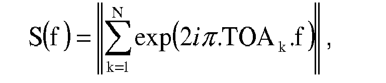
où f est une fréquence, N est le nombre d'impulsions dans le signal radar et TOAk sont les instants d'arrivée des impulsions, - une étape de séparation des trains d'impulsions à partir de leur FRI moyenne déterminées par la transformée de Fourier discrète.
- a step of determining a search range Δf c in which pulse repetition frequencies (FRI) are likely to be identified, this step comprising the following substeps:
- Constructing a histogram of arrival time differences (DTOA) comprising classes, each class being defined by a range of DTOA and including the pulses whose duration which separates them from the preceding pulses for a given order is within this range,
- Determining a search range Δt c bounded by the lower bound of the first class containing at least one pulse and by the upper bound of the last class containing at least one pulse,
- ■ determine a mean DTOA DTOA c as the average value of the search range Δt c ,
- Define a reference frequency f c as being equal to the inverse of the average DTOA c ,
the search range Δf c being defined in accordance with the relation:
or
- a step of calculating said discrete Fourier transform over the search range Δf c , according to the relation:
where f is a frequency, N is the number of pulses in the radar signal and TOA k are the arrival times of the pulses, - a step of separating the pulse trains from their average FRI determined by the discrete Fourier transform.
Le procédé peut comporter une étape préalable de détermination du pas d'échantillonnage δf pour la transformée de Fourier discrète, le pas d'échantillonnage vérifiant la relation : 
Selon une forme particulière de réalisation, la plage de recherche Δtc est définie par la borne inférieure de la première classe contenant un nombre d'impulsions supérieur ou égal à un seuil prédéterminé, et par la borne supérieure de la dernière classe contenant un nombre d'impulsions supérieur ou égal au seuil prédéterminé.According to one particular embodiment, the search range Δt c is defined by the lower bound of the first class containing a number of pulses greater than or equal to a predetermined threshold, and by the upper bound of the last class containing a number of pulses. impulses greater than or equal to the predetermined threshold.
Les classes de l'histogramme de DTOA peuvent avoir la même largeur de plage, cette largeur définit alors un pas d'histogramme ph, le pas d'histogramme ph étant déterminé de manière à être de l'ordre de 30 à 50 fois l'erreur de mesure et de quantification des instants d'arrivée TOAk des impulsions.The classes of the histogram of DTOA may have the same range width, this width then defines a histogram step p h , the histogram step p h being determined to be of the order of 30 to 50 times the measurement and quantization error of the arrival times TOA k pulses.
La plage de recherche Δfc peut en outre être limitée par une valeur minimale de borne inférieure fmin telle que : 
Selon une forme particulière de réalisation, seulement les composantes de la transformée de Fourier discrète (TFD) dont le module est supérieur à un seuil prédéterminé sTFD sont prises en compte pour la séparation des trains d'impulsions.According to a particular embodiment, only the components of the discrete Fourier transform (DFT) whose module is greater than a predetermined threshold s TFD are taken into account for the separation of the pulse trains.
Le seuil prédéterminé sTFD peut être déterminé par la relation suivante : sTFD = G(Jmax).(1-Tmmax).D.fRI, où Jmax est le taux de jitter maximal admissible pour le train d'impulsions, G(Jmax) est le gain de la TFD S(f) pour le taux de jitter maximal admissible Jmax, et Tmmax est le taux de mitage maximal admissible pour le train d'impulsions.The predetermined threshold s TFD can be determined by the following relation: s TFD = G (J max ). (1-Tm max ) .Df RI , where J max is the maximum allowable jitter rate for the pulse train, G (J max ) is the gain of TFD S (f) for the maximum allowable jitter rate J max , and Tm max is the maximum allowable spur rate for the pulse train.
L'invention a notamment pour avantage qu'elle permet d'utiliser le pouvoir séparateur de la transformée de Fourier sans nécessiter un coût de calcul important.The invention has the particular advantage that it allows to use the separating power of the Fourier transform without requiring a significant calculation cost.
L'invention sera mieux comprise et d'autres avantages apparaîtront à la lecture de la description détaillée d'un mode de réalisation donné à titre d'exemple, description faite en regard de dessins annexés qui représentent :
- la
figure 1 , des étapes possibles pour le procédé de séparation de trains d'impulsions selon l'invention ; - la
figure 2 , des histogrammes de différences de temps d'arrivée (DTOA) d'impulsions pour deux pas d'histogramme différents ; - la
figure 3 , un histogramme de DTOA pour un train d'impulsions avec une période de répétition des impulsions (PRI) fluctuant de 10% et la TFD calculée pour ce train d'impulsions ; - la
figure 4 , un exemple d'interpolation de la TFD autour de sa composante de plus forte amplitude ; - la
figure 5 , un histogramme de DTOA pour deux trains d'impulsions dont les PRI fluctuent de 10%, le premier train ayant une PRI moyenne de 100 µs et le deuxième train ayant une PRI moyenne de 102 µs ; - la
figure 6 , le gain pour les composantes de la TFD voisines de son pic principal en fonction du taux de fluctuation de la PRI ; - la
figure 7 , deux graphiques de phase tracés pour un signal radar comportant deux trains d'impulsions, le premier graphique donnant la phase du signal radar calculée à la PRI moyenne du premier train d'impulsions et le deuxième graphique donnant la phase du signal radar calculée à la PRI moyenne du deuxième train d'impulsions.
- the
figure 1 possible steps for the method of separating pulse trains according to the invention; - the
figure 2 pulse arrival time (DTOA) histograms for two different histogram pitches; - the
figure 3 , a DTOA histogram for a pulse train with a pulse repetition period (PRI) fluctuating by 10% and the calculated DFT for this pulse train; - the
figure 4 , an example of interpolation of the DFT around its higher amplitude component; - the
figure 5 , a histogram of DTOA for two pulse trains with PRIs fluctuating by 10%, the first train having an average PRI of 100 μs and the second train having an average PRI of 102 μs; - the
figure 6 , the gain for the components of the DFT close to its main peak as a function of the rate of fluctuation of the PRI; - the
figure 7 , two phase graphs plotted for a radar signal comprising two pulse trains, the first graph giving the phase of the radar signal calculated at the average PRI of the first pulse train and the second graph giving the phase of the radar signal calculated at the Average PRI of the second pulse train.
Pour la suite de la description, on considère un signal radar s(t), où t représente la variable temps. Le signal radar comporte N impulsions radar reçues et datées à leur arrivée pendant une durée d'acquisition D. Les impulsions radar sont par exemple reçues et datées par un récepteur de mesures. Chaque impulsion radar donne ainsi naissance à un instant d'arrivée TOAk, avec k compris entre 1 et N. Les impulsions peuvent provenir d'un unique émetteur ou de plusieurs émetteurs, chaque émetteur fournissant un train d'impulsion dont la période de répétition des impulsions (PRI) est susceptible de fluctuer autour d'une PRI moyenne. Un train d'impulsions dont la PRI fluctue est appelé train à PRI jittée.For the rest of the description, consider a radar signal s (t), where t represents the time variable. The radar signal comprises N radar pulses received and dated at their arrival during an acquisition period D. The radar pulses are for example received and dated by a receiver of measurements. Each radar pulse thus gives rise to a arrival time TOA k , with k being between 1 and N. The pulses can come from a single transmitter or from several transmitters, each transmitter providing a pulse train whose repetition period pulses (PRI) is likely to fluctuate around an average PRI. A pulse train whose PRI fluctuates is called a PRI train.
La
Le procédé de séparation de trains d'impulsions selon l'invention est basé sur le calcul de la transformée de Fourier discrète (TFD) appliquée aux instants d'arrivée TOAk des impulsions. Dans le cas d'un fonctionnement supervisé, c'est-à-dire lorsque la ou les fréquences de répétition des impulsions (FRI) du ou des trains d'impulsions sont connues a priori, la TFD peut n'être calculée qu'autour de cette ou de ces FRI. Le fonctionnement est par exemple supervisé lorsqu'un train d'impulsions a préalablement était détecté et caractérisé, et qu'il y a de fortes chances pour qu'il réapparaisse avec la même FRI. Au-delà de ce contexte de supervision, on cherche à déterminer une plage de fréquences dans laquelle des FRI sont susceptibles d'être identifiées. Cette plage de fréquences est appelée plage de recherche Δfc. Elle est par exemple centrée sur une fréquence de consigne fc.The method of separating pulse trains according to the invention is based on the calculation of the discrete Fourier transform (DFT) applied to the arrival times TOA k pulses. In the case of supervised operation, that is to say when the pulse repetition frequency or frequencies (FRI) of the pulse train or trains are known a priori, the DFT can be calculated only around this or these FRI. Operation is for example supervised when a pulse train has previously been detected and characterized, and there is a good chance that it will reappear with the same FRI. Beyond this supervision context, it is sought to determine a range of frequencies in which FRI are likely to be identified. This frequency range is called the search range Δf c . It is for example centered on a set frequency f c .
Selon l'invention, on détermine dans une première étape 101 la fréquence de consigne fc à partir d'un histogramme de différence de temps d'arrivée (DTOA). Des histogrammes de DTOA peuvent être construits pour différents ordres. Le réglage de l'ordre dépend du contexte d'utilisation de l'invention. Un histogramme de DTOA d'ordre m donné est construit en déterminant, pour chaque impulsion arrivée à l'instant TOAk, la durée la séparant de l'impulsion arrivée à l'instant TOAk-m, c'est-à-dire sa DTOA d'ordre m, et en regroupant les impulsions de DTOA voisines au sein de classes, chaque classe étant définie par une plage de DTOA et par un nombre d'impulsions. Toutes les classes peuvent avoir la même largeur de plage. La largeur de plage définit alors un pas d'histogramme ph. Avantageusement, le pas ph est choisi suffisamment large pour détecter un train d'impulsions à PRI jittée sur un faible nombre de classes adjacentes. En effet, si le pas d'histogramme ph est trop fin, les DTOA risquent d'être réparties sur de nombreuses classes non adjacentes. II est alors difficile de différencier les classes pertinentes, c'est-à-dire celles contenant des DTOA correspondant effectivement à une valeur de PRI, des classes formées par le bruit, par exemple du fait d'impulsions manquantes. A l'inverse, le pas d'histogramme ph ne pas ne doit pas être trop large pour éviter le regroupement de toutes les impulsions dans une seule classe. Selon une forme particulière de réalisation, le pas d'histogramme ph est déterminé de manière à être de l'ordre de 30 à 50 fois cette erreur pour la détection de trains d'impulsions à PRI jittée. La plage de recherche Δfc pour le calcul de la TFD peut ainsi être déterminée à partir des classes de l'histogramme. En l'occurrence, on peut considérer une plage de recherche Δtc dans le domaine temporel (DTOA) définie par la borne inférieure de la première classe contenant au moins une impulsion et par la borne supérieure de la dernière classe contenant au moins une impulsion. La DTOA moyenne de la plage de recherche Δtc est appelée DTOA de consigne DTOAc. La moyenne considérée est par exemple la moyenne arithmétique. La fréquence de consigne fc est alors définie par l'inverse de cette DTOA de consigne DTOAc. La TFD est calculée autour de cette fréquence fc sur la plage de recherche Δfc.According to the invention, the set frequency f c is determined in a
Avantageusement, seulement les classes dont le nombre d'occurrences dépasse un seuil prédéterminé sont prises en compte pour la détermination de la plage de recherche Δtc. La plage de recherche Δtc est alors bornée par une DTOA minimale correspondant à la borne inférieure de la première classe contenant un nombre d'impulsions supérieur ou égal au seuil et par une DTOA maximale correspondant à la borne supérieure de la dernière classe contenant un nombre d'impulsions supérieur ou égal au seuil. Les classes contenant un nombre d'impulsions inférieur au seuil peuvent être considérées comme ne contenant aucune impulsion. Selon une forme particulière de réalisation de l'invention, si deux classes contenant un nombre d'impulsions supérieur ou égal au seuil sont séparées par au moins deux classes contenant un nombre d'impulsions inférieur au seuil, on considère deux plages de recherche distinctes Δtc1 et Δtc2.Advantageously, only the classes whose number of occurrences exceeds a predetermined threshold are taken into account for the determination of the search range Δt c . The search range Δt c is then bounded by a minimum DTOA corresponding to the lower bound of the first class containing a number of pulses greater than or equal to the threshold and by a maximum DTOA corresponding to the upper bound of the last class containing a number pulses greater than or equal to the threshold. Classes containing a number of pulses below the threshold may be considered as containing no pulse. According to a particular embodiment of the invention, if two classes containing a number of pulses greater than or equal to the threshold are separated by at least two classes containing a number of pulses less than the threshold, two distinct search ranges Δt are considered. c1 and Δt c2 .
La
La fréquence de consigne fc ayant été déterminée, il reste notamment à déterminer le pas d'échantillonnage δf des fréquences de calcul pour la transformée de Fourier discrète. La détermination du pas d'échantillonnage δf fait l'objet de l'étape 102. Avec une durée d'acquisition des impulsions radar d'une durée D, la TFD calculée sur les TOAk des impulsions présente une largeur de lobe autour de la FRI moyenne au minimum égale à 2/D. En effet, lorsque la première et la dernière impulsion appartiennent à un même train d'impulsions, la durée effective du train d'impulsions est égale à D. La largeur du lobe principal de la TFD est alors égale à 2/D. En revanche, en présence de deux ou plusieurs trains d'impulsions imbriqués, la durée effective de l'un des trains d'impulsions peut être plus faible et donc le lobe principal de sa TFD peut être plus large que 2/D. A titre d'exemple, dans un signal radar de durée D contenant le mélange d'un train T1 de durée D1=D/2 et d'un train T2 de durée D2=D, le train T1 n'est présent qu'une partie de D et donc le lobe de la TF relatif à sa PRI aura une largeur de 4/D, bien plus large que celle à laquelle on pouvait s'attendre.Since the reference frequency f c has been determined, it remains in particular to determine the sampling step δf of the calculation frequencies for the discrete Fourier transform. The determination of the sampling step δf is the subject of
Afin de ne manquer aucun pic de la TFD, le pas d'échantillonnage δf des fréquences de calcul doit être suffisamment petit. II est par exemple fixé à la valeur inverse de la durée d'acquisition D du signal radar : 
La plage de recherche Δfc pour le calcul de la transformée de Fourier discrète peut être déterminée dans l'étape 103 à partir de la fréquence de consigne fc et du pas d'échantillonnage δf, conformément à la relation suivante : ![]()
avec 
![]()
with
La plage de fréquences Δfc peut également être exprimée en pourcentage P du DTOA de consigne DTOAc. Dans ce cas, la relation 2.1 devient : 
II est à noter que la résolution en fréquence δf de la TFD du signal radar s(t) étant constante sur toute la plage de recherche Δfc dans le domaine fréquentiel, la résolution en PRI δpri ne l'est pas. En particulier, pour une résolution en fréquence δf égale à 1/D, la résolution en PRI δpri est : 
La relation 3 montre que lorsque la PRI est grande, la résolution en PRI peut devenir insuffisante. II existe donc une PRI limite PRImax au-delà de laquelle la TFD n'a plus une résolution suffisante. En raison du pouvoir concentrateur de la TFD, sa résolution est la plus grossière pour les faibles taux de jitter. La PRI limite PRImax est donc calculée par rapport au pourcentage minimal de jitter Qmin que l'on pense observer dans le signal radar : 
Dans le domaine fréquentiel, elle correspond à une fréquence minimale fmin au-dessous de laquelle il n'est pas nécessaire de calculer la TFD. Cette fréquence minimale fmin est égale à l'inverse de PRImax. Elle permet donc de limiter la plage de recherche Δfc définie à la relation 2.In the frequency domain, it corresponds to a minimum frequency f min below which it is not necessary to calculate the DFT. This minimum frequency f min is equal to the inverse of PRI max . It therefore makes it possible to limit the search range Δf c defined in
Par ailleurs, le domaine d'application de la TFD peut être limité en fonction du nombre Nmin d'impulsions dans le signal radar. La TFD ne devrait normalement pas être calculée pour des fréquences correspondant à des PRI supérieures à D/Nmin.Moreover, the field of application of the DFT can be limited according to the number N min of pulses in the radar signal. The DFT should not normally be calculated for frequencies corresponding to PRI greater than D / N min .
D'une manière générale, pour pouvoir estimer correctement un taux de jitter d'une PRI de ± J/2 % avec une TFD, il est nécessaire de disposer d'au moins 100/J impulsions. A titre d'exemple, il faut au moins 10 impulsions pour estimer correctement, avec la TFD, une PRI jittée de plus ou moins 5 %, ou il faut au moins 20 impulsions pour une PRI jittée de plus ou moins 2,5 %.In general, to be able to correctly estimate a jitter rate of a PRI of ± J / 2% with a DFT, it is necessary to have at least 100 / J pulses. By way of example, it takes at least 10 pulses to correctly estimate, with the DFT, a PRI jittered by plus or minus 5%, or it takes at least 20 pulses for a PRI jittered by plus or minus 2.5%.
Dans une quatrième étape 104, on calcule la transformée de Fourier discrète S(f) du signal radar s(t) pour les instants d'arrivée TOAk des impulsions. Les composantes de la TFD S(f) sont calculées pour des fréquences f comprises dans la plage de recherche Δfc déterminée dans l'étape 103 avec le pas d'échantillonnage δf déterminé lors de l'étape 102, conformément à la relation suivante : 
La
La composante 42 de plus forte amplitude ne correspond pas forcément au maximum de la transformée de Fourier non échantillonnée. Or même un écart très faible sur l'estimation de la FRI moyenne peut être gênant pour la suite du procédé. Afin de réduire cette erreur, il est possible d'interpoler la TFD autour de sa composante 42 de plus forte amplitude. La TFD peut par exemple être interpolée par une expression parabolique simple du fait de la forme pratiquement parabolique du pic principal. La
La
La
Une fois que la TFD a été calculée sur la plage de recherche Δfc, il est possible de s'assurer que son maximum correspond bien à la FRI du signal radar s(t). A cet effet, le maximum de la TFD peut être comparé à un seuil sTFD dans une cinquième étape 105. Théoriquement, un train d'impulsions de fréquence de répétition des impulsions fRI observé sur une durée D donne un nombre d'impulsions égal au produit D.fRI. Afin de prendre en compte l'absence d'impulsions, le produit D.fRI peut être pondéré par un coefficient de pondération. Ce coefficient prend par exemple en compte le taux de mitage maximal admissible Tmmax ainsi que le gain G de la TFD S(f) en fonction du taux de jitter maximal admissible Jmax (représenté sur la ![]()
![]()
Par mitage, on entend le manque d'une ou plusieurs impulsions dans un train d'impulsions, par exemple dû à la non réception de cette ou de ces impulsions. Le taux de mitage est le pourcentage d'impulsions manquantes d'un train par rapport au nombre total d'impulsions de ce train. A titre d'exemple, pour un taux de jitter maximal admissible Jmax de 40%, correspondant à un gain G de 0,75, et un taux de mitage maximal admissible Tmmax de 60%, le coefficient de pondération est égal à 0,3.By mitage means the lack of one or more pulses in a pulse train, for example due to the non-receipt of this or these pulses. The rate of mourning is the percentage of missing pulses of a train compared to the total number of pulses of this train. For example, for a maximum allowable jitter rate J max of 40%, corresponding to a G gain of 0.75, and a maximum permissible mite rate Tm max of 60%, the weighting coefficient is equal to 0 3.
On peut ajouter à ce seuil un élément de dénombrement des impulsions appartenant à un train en fixant un nombre minimal d'impulsions Nmin. Ce nombre Nmin est un réglage opérationnel. II est par exemple égal à cinq. Le seuil devient alors : ![]()
![]()
Lorsqu'un signal radar comporte des impulsions appartenant à différents trains, c'est-à-dire provenant d'émetteurs différents, l'histogramme de DTOA construit dans l'étape 101 présente des classes disjointes ou non. Si les PRI des trains sont suffisamment différentes les unes des autres, les classes de l'histogramme forment des groupes de classes disjoints. Les impulsions de chaque train peuvent alors être séparées en fonction du groupe de classe auquel elles appartiennent. II n'est alors pas nécessaire de calculer la TFD sur les TOAk de ces impulsions. En revanche, si les PRI des différents trains fluctuent et sont proches, les classes de l'histogramme ne forment qu'un seul groupe n'offrant donc plus de résolution. La TFD peut alors être calculée sur les TOAk des impulsions conformément à l'étape 104. La TFD permet d'observer deux pics disjoints lorsque l'écart de PRI est suffisamment grand par rapport à son pouvoir séparateur. Ses différents pics principaux permettent de déterminer précisément la PRI moyenne de chaque train d'impulsions. Cette connaissance permet alors, dans une étape 106, de séparer les impulsions relativement au train auquel elles appartiennent.When a radar signal comprises pulses belonging to different trains, that is to say from different transmitters, the histogram of DTOA built in
Selon une forme particulière de réalisation, la séparation des trains d'impulsions est effectuée en analysant la phase des impulsions. On entend par phase Φk d'une impulsion relativement à une PRI donnée, la quantité : ![]()
où l'opérateur mod définit le modulo.
Les impulsions appartenant à un même train ayant des instants d'arrivée TOAk successifs séparés par une durée sensiblement égale à la PRI moyenne de ce train, leur phase Φk est sensiblement constante sur toute la durée d'acquisition D du signal radar lorsqu'elle est calculée pour cette PRI moyenne. La phase peut ne pas être tout à fait constante du fait de la fluctuation de la PRI. Cependant, la phase évolue dans ce cas autour d'une valeur moyenne. En revanche, lorsque la phase Φk est calculée pour une PRI ne correspondant pas à la PRI moyenne d'un train, il n'y a pas de cohérence dans les instants d'arrivée TOAk des impulsions de ce train. La phase de ces impulsions n'est donc pas constante. Par conséquent, les impulsions dont la phase est constante peuvent être séparées et identifiées comme appartenant à un train dont la PRI moyenne est celle utilisée pour le calcul de la phase.According to a particular embodiment, the separation of the pulse trains is performed by analyzing the phase of the pulses. Phase Φ k of an impulse relative to a given PRI, the quantity: ![]()
where the mod operator defines the modulo.
The pulses belonging to the same train having successive arrival times TOA k separated by a duration substantially equal to the average PRI of this train, their phase Φ k is substantially constant over the duration of acquisition D of the radar signal when it is calculated for this average PRI. The phase may not be quite constant due to the fluctuation of the PRI. However, the phase evolves in this case around an average value. On the other hand, when the phase Φk is calculated for a PRI that does not correspond to the average PRI of a train, there is no coherence in the arrival times TOA k of the pulses of this train. The phase of these pulses is therefore not constant. Therefore, the pulses whose phase is constant can be separated and identified as belonging to a train whose average PRI is the one used for the calculation of the phase.
La
A la fin de l'étape 106, lorsqu'un ou plusieurs trains ont été séparés, le procédé de séparation des trains d'impulsions peut être réitéré à partir de l'étape 101. Chaque nouvelle itération est susceptible d'entraîner le calcul d'une TFD avec une plage de recherche en fréquence et un pas d'échantillonnage différents. La nouvelle TFD peut être mieux adaptée aux impulsions restantes.At the end of
Claims (7)
la plage de recherche Δfc étant définie conformément à la relation :
où


où f est une fréquence, N est le nombre d'impulsions dans le signal radar et TOAk sont les instants d'arrivée des impulsions,
the search range Δf c being defined in accordance with the relation:
or
where f is a frequency, N is the number of pulses in the radar signal and TOA k are the arrival times of the pulses,


où Qmin est le pourcentage minimal de jitter que l'on pense observer pour les trains d'impulsions du signal radar.Method according to one of the preceding claims, characterized in that the search range Δf c is limited by a minimum lower limit value f min such that:
where Q min is the minimum percentage of jitter that is expected to be observed for pulse trains of the radar signal.
où Jmax est le taux de jitter maximal admissible pour le train d'impulsions, G(Jmax) est le gain de la transformée de Fourrier discrète S(f) pour le taux de jitter maximal admissible Jmax, et Tmmax est le taux de mitage maximal admissible pour le train d'impulsions.Method according to Claim 6, characterized in that the predetermined threshold s TFD is determined by the following relation:
where J max is the maximum allowable jitter rate for the pulse train, G (J max ) is the gain of the discrete Fourier transform S (f) for the maximum allowable jitter rate J max , and Tm max is the maximum permissible dust rate for the pulse train.
Applications Claiming Priority (1)
| Application Number | Priority Date | Filing Date | Title |
|---|---|---|---|
| FR0904600A FR2950701B1 (en) | 2009-09-25 | 2009-09-25 | METHOD FOR SEPARATING IMBRITIC RADAR PULSE TRAINS |
Publications (2)
| Publication Number | Publication Date |
|---|---|
| EP2309289A1 true EP2309289A1 (en) | 2011-04-13 |
| EP2309289B1 EP2309289B1 (en) | 2012-03-28 |
Family
ID=42109822
Family Applications (1)
| Application Number | Title | Priority Date | Filing Date |
|---|---|---|---|
| EP10176487A Active EP2309289B1 (en) | 2009-09-25 | 2010-09-13 | Method for separating interleaved radar puls sequences |
Country Status (3)
| Country | Link |
|---|---|
| EP (1) | EP2309289B1 (en) |
| AT (1) | ATE551617T1 (en) |
| FR (1) | FR2950701B1 (en) |
Cited By (6)
| Publication number | Priority date | Publication date | Assignee | Title |
|---|---|---|---|---|
| CN105807264A (en) * | 2016-03-28 | 2016-07-27 | 中国航空工业集团公司雷华电子技术研究所 | Method for detecting radar pulse repetition frequency and estimating inceptive pulse arrival time |
| WO2017198860A1 (en) * | 2016-05-20 | 2017-11-23 | Thales | Method of processing a signal formed of a sequence of pulses |
| WO2018002208A1 (en) * | 2016-06-30 | 2018-01-04 | Thales | Method for estimating an average arrival date for a train of pulses |
| CN109190303A (en) * | 2018-10-15 | 2019-01-11 | 西安电子工程研究所 | Middle short range search radar emits signal width pulse width ratio design method |
| CN114417943A (en) * | 2022-03-29 | 2022-04-29 | 中国科学院空天信息创新研究院 | Identification method of repetition frequency modulation type |
| WO2022189298A1 (en) * | 2021-03-11 | 2022-09-15 | Thales | Method for fast and robust deinterleaving of pulse trains |
Citations (3)
| Publication number | Priority date | Publication date | Assignee | Title |
|---|---|---|---|---|
| US5396250A (en) | 1992-12-03 | 1995-03-07 | The United States Of America As Represented By The Secretary Of The Air Force | Spectral estimation of radar time-of-arrival periodicities |
| US5583505A (en) * | 1995-09-11 | 1996-12-10 | Lockheed Martin Corporation | Radar pulse detection and classification system |
| US7397415B1 (en) * | 2006-02-02 | 2008-07-08 | Itt Manufacturing Enterprises, Inc. | System and method for detecting and de-interleaving radar emitters |
-
2009
- 2009-09-25 FR FR0904600A patent/FR2950701B1/en not_active Expired - Fee Related
-
2010
- 2010-09-13 AT AT10176487T patent/ATE551617T1/en active
- 2010-09-13 EP EP10176487A patent/EP2309289B1/en active Active
Patent Citations (3)
| Publication number | Priority date | Publication date | Assignee | Title |
|---|---|---|---|---|
| US5396250A (en) | 1992-12-03 | 1995-03-07 | The United States Of America As Represented By The Secretary Of The Air Force | Spectral estimation of radar time-of-arrival periodicities |
| US5583505A (en) * | 1995-09-11 | 1996-12-10 | Lockheed Martin Corporation | Radar pulse detection and classification system |
| US7397415B1 (en) * | 2006-02-02 | 2008-07-08 | Itt Manufacturing Enterprises, Inc. | System and method for detecting and de-interleaving radar emitters |
Non-Patent Citations (1)
| Title |
|---|
| MARDIA H K: "NEW TECHNIQUES FOR THE DEINTERLEAVING OF REPETITIVE SEQUENCES", IEE PROCEEDINGS F. COMMUNICATIONS, RADAR & SIGNALPROCESSING, INSTITUTION OF ELECTRICAL ENGINEERS. STEVENAGE, GB, vol. 136, no. 4, PART F, 1 August 1989 (1989-08-01), pages 149 - 154, XP000052595, ISSN: 0956-375X * |
Cited By (13)
| Publication number | Priority date | Publication date | Assignee | Title |
|---|---|---|---|---|
| CN105807264B (en) * | 2016-03-28 | 2018-02-27 | 中国航空工业集团公司雷华电子技术研究所 | Radar pulse repetition frequency detects the method for estimation with inceptive impulse arrival time |
| CN105807264A (en) * | 2016-03-28 | 2016-07-27 | 中国航空工业集团公司雷华电子技术研究所 | Method for detecting radar pulse repetition frequency and estimating inceptive pulse arrival time |
| US10935648B2 (en) | 2016-05-20 | 2021-03-02 | Thales | Method of processing a signal formed of a sequence of pulses |
| WO2017198860A1 (en) * | 2016-05-20 | 2017-11-23 | Thales | Method of processing a signal formed of a sequence of pulses |
| FR3051611A1 (en) * | 2016-05-20 | 2017-11-24 | Thales Sa | METHOD FOR PROCESSING A SIGNAL FORM OF A PULSE SEQUENCE |
| WO2018002208A1 (en) * | 2016-06-30 | 2018-01-04 | Thales | Method for estimating an average arrival date for a train of pulses |
| FR3053475A1 (en) * | 2016-06-30 | 2018-01-05 | Thales | METHOD OF ESTIMATING AN AVERAGE ARRIVAL DATE OF A PULSE TRAIN |
| CN109190303A (en) * | 2018-10-15 | 2019-01-11 | 西安电子工程研究所 | Middle short range search radar emits signal width pulse width ratio design method |
| CN109190303B (en) * | 2018-10-15 | 2023-04-07 | 西安电子工程研究所 | Method for designing width-to-width pulse width ratio of medium-short range search radar transmitted signal |
| WO2022189298A1 (en) * | 2021-03-11 | 2022-09-15 | Thales | Method for fast and robust deinterleaving of pulse trains |
| FR3120762A1 (en) * | 2021-03-11 | 2022-09-16 | Thales | METHOD FOR RAPID AND ROBUST DEINTERLACING OF PULSE TRAINS |
| CN114417943A (en) * | 2022-03-29 | 2022-04-29 | 中国科学院空天信息创新研究院 | Identification method of repetition frequency modulation type |
| CN114417943B (en) * | 2022-03-29 | 2022-06-10 | 中国科学院空天信息创新研究院 | Identification method of repetition frequency modulation type |
Also Published As
| Publication number | Publication date |
|---|---|
| ATE551617T1 (en) | 2012-04-15 |
| EP2309289B1 (en) | 2012-03-28 |
| FR2950701B1 (en) | 2011-10-21 |
| FR2950701A1 (en) | 2011-04-01 |
Similar Documents
| Publication | Publication Date | Title |
|---|---|---|
| EP2309289B1 (en) | Method for separating interleaved radar puls sequences | |
| EP3008479B1 (en) | Reflectometry method for identifying soft faults affecting a cable | |
| EP1982209B1 (en) | Frequency measuring broadband digital receiver | |
| EP2834653B1 (en) | Method and system for diagnosing a cable by distributed reflectometry with selective averaging | |
| EP1097354B1 (en) | Crossed measurements of flowmeter sound signals | |
| FR2901366A1 (en) | METHOD FOR DETECTING REFLECTORS OF ELECTROMAGNETIC IMPLUSION | |
| EP3811109B1 (en) | Method for measuring wave height by means of an airborne radar | |
| EP3259608B1 (en) | Method for characterising an unclear fault in a cable | |
| EP2366118B1 (en) | Wideband digital receiver comprising a phase jump detection mechanism | |
| EP3645981B1 (en) | Method for measuring a speed of a fluid | |
| FR3050849B1 (en) | METHOD AND DEVICE FOR REDUCING NOISE IN A MODULE SIGNAL | |
| EP1940023A2 (en) | Bank of cascadable digital filters, and reception circuit including such a bank of cascaded filters | |
| EP2453261B1 (en) | Method for GNSS signal distortion detection | |
| EP2366117B1 (en) | Wideband digital receiver comprising a signal detection mechanism | |
| FR2946149A1 (en) | Electrical cable analyzing method for electrical system, involves injecting probe signal with total duration in cable, and locating reference measurement point selected on measurement of injected signal at center of middle portion of signal | |
| EP3605145B1 (en) | High-resolution remote processing method | |
| WO2015144649A1 (en) | Method for detection of a target signal in a measurement signal of an instrument installed on a spacecraft engine, and measurement system | |
| EP3516769B1 (en) | Device for generating a continuous carrier signal from a reference pulse signal | |
| EP3516414B1 (en) | Device for generating a continuous carrier signal from a reference pulse signal | |
| EP3877773B1 (en) | System for analysing faults by reflectometry of optimised dynamic range | |
| EP1995565B1 (en) | Device for processing signals from systems with differential configuration | |
| EP3538917B1 (en) | Method for testing the electromagnetic compatibility of a radar detector with at least one onboard pulse signal transmitter | |
| FR2972055A1 (en) | Method for determination of row of distance ambiguity of echo signal received by Doppler type pulsed radar, involves determining row of distance ambiguity of echo signal from one of three frequency spectrums | |
| FR2998973A1 (en) | Method for determining characteristics of radar signal in presence of interferences for electromagnetic environmental monitoring application, involves eliminating values of differences in times of arrival that are out of agility fields | |
| FR3090105A1 (en) | Method for detecting leaks in a resource distribution network |
Legal Events
| Date | Code | Title | Description |
|---|---|---|---|
| PUAI | Public reference made under article 153(3) epc to a published international application that has entered the european phase |
Free format text: ORIGINAL CODE: 0009012 |
|
| AK | Designated contracting states |
Kind code of ref document: A1 Designated state(s): AL AT BE BG CH CY CZ DE DK EE ES FI FR GB GR HR HU IE IS IT LI LT LU LV MC MK MT NL NO PL PT RO SE SI SK SM TR |
|
| AX | Request for extension of the european patent |
Extension state: BA ME RS |
|
| 17P | Request for examination filed |
Effective date: 20110915 |
|
| GRAP | Despatch of communication of intention to grant a patent |
Free format text: ORIGINAL CODE: EPIDOSNIGR1 |
|
| RTI1 | Title (correction) |
Free format text: METHOD FOR SEPARATING INTERLEAVED RADAR PULS SEQUENCES |
|
| GRAS | Grant fee paid |
Free format text: ORIGINAL CODE: EPIDOSNIGR3 |
|
| GRAA | (expected) grant |
Free format text: ORIGINAL CODE: 0009210 |
|
| AK | Designated contracting states |
Kind code of ref document: B1 Designated state(s): AL AT BE BG CH CY CZ DE DK EE ES FI FR GB GR HR HU IE IS IT LI LT LU LV MC MK MT NL NO PL PT RO SE SI SK SM TR |
|
| REG | Reference to a national code |
Ref country code: GB Ref legal event code: FG4D Free format text: NOT ENGLISH |
|
| REG | Reference to a national code |
Ref country code: CH Ref legal event code: EP |
|
| REG | Reference to a national code |
Ref country code: AT Ref legal event code: REF Ref document number: 551617 Country of ref document: AT Kind code of ref document: T Effective date: 20120415 |
|
| REG | Reference to a national code |
Ref country code: IE Ref legal event code: FG4D Free format text: LANGUAGE OF EP DOCUMENT: FRENCH |
|
| REG | Reference to a national code |
Ref country code: DE Ref legal event code: R096 Ref document number: 602010001202 Country of ref document: DE Effective date: 20120524 |
|
| REG | Reference to a national code |
Ref country code: NL Ref legal event code: VDEP Effective date: 20120328 |
|
| PG25 | Lapsed in a contracting state [announced via postgrant information from national office to epo] |
Ref country code: LT Free format text: LAPSE BECAUSE OF FAILURE TO SUBMIT A TRANSLATION OF THE DESCRIPTION OR TO PAY THE FEE WITHIN THE PRESCRIBED TIME-LIMIT Effective date: 20120328 Ref country code: NO Free format text: LAPSE BECAUSE OF FAILURE TO SUBMIT A TRANSLATION OF THE DESCRIPTION OR TO PAY THE FEE WITHIN THE PRESCRIBED TIME-LIMIT Effective date: 20120628 Ref country code: HR Free format text: LAPSE BECAUSE OF FAILURE TO SUBMIT A TRANSLATION OF THE DESCRIPTION OR TO PAY THE FEE WITHIN THE PRESCRIBED TIME-LIMIT Effective date: 20120328 |
|
| LTIE | Lt: invalidation of european patent or patent extension |
Effective date: 20120328 |
|
| PG25 | Lapsed in a contracting state [announced via postgrant information from national office to epo] |
Ref country code: FI Free format text: LAPSE BECAUSE OF FAILURE TO SUBMIT A TRANSLATION OF THE DESCRIPTION OR TO PAY THE FEE WITHIN THE PRESCRIBED TIME-LIMIT Effective date: 20120328 Ref country code: GR Free format text: LAPSE BECAUSE OF FAILURE TO SUBMIT A TRANSLATION OF THE DESCRIPTION OR TO PAY THE FEE WITHIN THE PRESCRIBED TIME-LIMIT Effective date: 20120629 Ref country code: LV Free format text: LAPSE BECAUSE OF FAILURE TO SUBMIT A TRANSLATION OF THE DESCRIPTION OR TO PAY THE FEE WITHIN THE PRESCRIBED TIME-LIMIT Effective date: 20120328 |
|
| REG | Reference to a national code |
Ref country code: AT Ref legal event code: MK05 Ref document number: 551617 Country of ref document: AT Kind code of ref document: T Effective date: 20120328 |
|
| PG25 | Lapsed in a contracting state [announced via postgrant information from national office to epo] |
Ref country code: CY Free format text: LAPSE BECAUSE OF FAILURE TO SUBMIT A TRANSLATION OF THE DESCRIPTION OR TO PAY THE FEE WITHIN THE PRESCRIBED TIME-LIMIT Effective date: 20120328 |
|
| PG25 | Lapsed in a contracting state [announced via postgrant information from national office to epo] |
Ref country code: EE Free format text: LAPSE BECAUSE OF FAILURE TO SUBMIT A TRANSLATION OF THE DESCRIPTION OR TO PAY THE FEE WITHIN THE PRESCRIBED TIME-LIMIT Effective date: 20120328 Ref country code: IS Free format text: LAPSE BECAUSE OF FAILURE TO SUBMIT A TRANSLATION OF THE DESCRIPTION OR TO PAY THE FEE WITHIN THE PRESCRIBED TIME-LIMIT Effective date: 20120728 Ref country code: SE Free format text: LAPSE BECAUSE OF FAILURE TO SUBMIT A TRANSLATION OF THE DESCRIPTION OR TO PAY THE FEE WITHIN THE PRESCRIBED TIME-LIMIT Effective date: 20120328 Ref country code: RO Free format text: LAPSE BECAUSE OF FAILURE TO SUBMIT A TRANSLATION OF THE DESCRIPTION OR TO PAY THE FEE WITHIN THE PRESCRIBED TIME-LIMIT Effective date: 20120328 Ref country code: PL Free format text: LAPSE BECAUSE OF FAILURE TO SUBMIT A TRANSLATION OF THE DESCRIPTION OR TO PAY THE FEE WITHIN THE PRESCRIBED TIME-LIMIT Effective date: 20120328 Ref country code: SI Free format text: LAPSE BECAUSE OF FAILURE TO SUBMIT A TRANSLATION OF THE DESCRIPTION OR TO PAY THE FEE WITHIN THE PRESCRIBED TIME-LIMIT Effective date: 20120328 Ref country code: CZ Free format text: LAPSE BECAUSE OF FAILURE TO SUBMIT A TRANSLATION OF THE DESCRIPTION OR TO PAY THE FEE WITHIN THE PRESCRIBED TIME-LIMIT Effective date: 20120328 |
|
| PG25 | Lapsed in a contracting state [announced via postgrant information from national office to epo] |
Ref country code: PT Free format text: LAPSE BECAUSE OF FAILURE TO SUBMIT A TRANSLATION OF THE DESCRIPTION OR TO PAY THE FEE WITHIN THE PRESCRIBED TIME-LIMIT Effective date: 20120730 Ref country code: SK Free format text: LAPSE BECAUSE OF FAILURE TO SUBMIT A TRANSLATION OF THE DESCRIPTION OR TO PAY THE FEE WITHIN THE PRESCRIBED TIME-LIMIT Effective date: 20120328 |
|
| PG25 | Lapsed in a contracting state [announced via postgrant information from national office to epo] |
Ref country code: NL Free format text: LAPSE BECAUSE OF FAILURE TO SUBMIT A TRANSLATION OF THE DESCRIPTION OR TO PAY THE FEE WITHIN THE PRESCRIBED TIME-LIMIT Effective date: 20120328 Ref country code: AT Free format text: LAPSE BECAUSE OF FAILURE TO SUBMIT A TRANSLATION OF THE DESCRIPTION OR TO PAY THE FEE WITHIN THE PRESCRIBED TIME-LIMIT Effective date: 20120328 Ref country code: DK Free format text: LAPSE BECAUSE OF FAILURE TO SUBMIT A TRANSLATION OF THE DESCRIPTION OR TO PAY THE FEE WITHIN THE PRESCRIBED TIME-LIMIT Effective date: 20120328 |
|
| PLBE | No opposition filed within time limit |
Free format text: ORIGINAL CODE: 0009261 |
|
| STAA | Information on the status of an ep patent application or granted ep patent |
Free format text: STATUS: NO OPPOSITION FILED WITHIN TIME LIMIT |
|
| 26N | No opposition filed |
Effective date: 20130103 |
|
| BERE | Be: lapsed |
Owner name: THALES Effective date: 20120930 |
|
| REG | Reference to a national code |
Ref country code: DE Ref legal event code: R097 Ref document number: 602010001202 Country of ref document: DE Effective date: 20130103 |
|
| PG25 | Lapsed in a contracting state [announced via postgrant information from national office to epo] |
Ref country code: ES Free format text: LAPSE BECAUSE OF FAILURE TO SUBMIT A TRANSLATION OF THE DESCRIPTION OR TO PAY THE FEE WITHIN THE PRESCRIBED TIME-LIMIT Effective date: 20120709 Ref country code: MC Free format text: LAPSE BECAUSE OF NON-PAYMENT OF DUE FEES Effective date: 20120930 |
|
| REG | Reference to a national code |
Ref country code: IE Ref legal event code: MM4A |
|
| PG25 | Lapsed in a contracting state [announced via postgrant information from national office to epo] |
Ref country code: BG Free format text: LAPSE BECAUSE OF FAILURE TO SUBMIT A TRANSLATION OF THE DESCRIPTION OR TO PAY THE FEE WITHIN THE PRESCRIBED TIME-LIMIT Effective date: 20120628 Ref country code: DE Free format text: LAPSE BECAUSE OF NON-PAYMENT OF DUE FEES Effective date: 20130403 Ref country code: IE Free format text: LAPSE BECAUSE OF NON-PAYMENT OF DUE FEES Effective date: 20120913 Ref country code: BE Free format text: LAPSE BECAUSE OF NON-PAYMENT OF DUE FEES Effective date: 20120930 |
|
| REG | Reference to a national code |
Ref country code: DE Ref legal event code: R119 Ref document number: 602010001202 Country of ref document: DE Effective date: 20130403 |
|
| PG25 | Lapsed in a contracting state [announced via postgrant information from national office to epo] |
Ref country code: AL Free format text: LAPSE BECAUSE OF FAILURE TO SUBMIT A TRANSLATION OF THE DESCRIPTION OR TO PAY THE FEE WITHIN THE PRESCRIBED TIME-LIMIT Effective date: 20120328 Ref country code: MT Free format text: LAPSE BECAUSE OF FAILURE TO SUBMIT A TRANSLATION OF THE DESCRIPTION OR TO PAY THE FEE WITHIN THE PRESCRIBED TIME-LIMIT Effective date: 20120328 |
|
| PG25 | Lapsed in a contracting state [announced via postgrant information from national office to epo] |
Ref country code: TR Free format text: LAPSE BECAUSE OF FAILURE TO SUBMIT A TRANSLATION OF THE DESCRIPTION OR TO PAY THE FEE WITHIN THE PRESCRIBED TIME-LIMIT Effective date: 20120328 |
|
| PG25 | Lapsed in a contracting state [announced via postgrant information from national office to epo] |
Ref country code: LU Free format text: LAPSE BECAUSE OF NON-PAYMENT OF DUE FEES Effective date: 20120913 Ref country code: SM Free format text: LAPSE BECAUSE OF FAILURE TO SUBMIT A TRANSLATION OF THE DESCRIPTION OR TO PAY THE FEE WITHIN THE PRESCRIBED TIME-LIMIT Effective date: 20120328 |
|
| PG25 | Lapsed in a contracting state [announced via postgrant information from national office to epo] |
Ref country code: HU Free format text: LAPSE BECAUSE OF FAILURE TO SUBMIT A TRANSLATION OF THE DESCRIPTION OR TO PAY THE FEE WITHIN THE PRESCRIBED TIME-LIMIT Effective date: 20100913 |
|
| REG | Reference to a national code |
Ref country code: CH Ref legal event code: PL |
|
| PG25 | Lapsed in a contracting state [announced via postgrant information from national office to epo] |
Ref country code: CH Free format text: LAPSE BECAUSE OF NON-PAYMENT OF DUE FEES Effective date: 20140930 Ref country code: MK Free format text: LAPSE BECAUSE OF FAILURE TO SUBMIT A TRANSLATION OF THE DESCRIPTION OR TO PAY THE FEE WITHIN THE PRESCRIBED TIME-LIMIT Effective date: 20120328 Ref country code: LI Free format text: LAPSE BECAUSE OF NON-PAYMENT OF DUE FEES Effective date: 20140930 |
|
| REG | Reference to a national code |
Ref country code: FR Ref legal event code: PLFP Year of fee payment: 7 |
|
| REG | Reference to a national code |
Ref country code: FR Ref legal event code: PLFP Year of fee payment: 8 |
|
| REG | Reference to a national code |
Ref country code: FR Ref legal event code: PLFP Year of fee payment: 9 |
|
| P01 | Opt-out of the competence of the unified patent court (upc) registered |
Effective date: 20230516 |
|
| PGFP | Annual fee paid to national office [announced via postgrant information from national office to epo] |
Ref country code: IT Payment date: 20230829 Year of fee payment: 14 Ref country code: GB Payment date: 20230817 Year of fee payment: 14 |
|
| PGFP | Annual fee paid to national office [announced via postgrant information from national office to epo] |
Ref country code: FR Payment date: 20230821 Year of fee payment: 14 |