EP2088281A1 - Method for determining the viscosity of a waxy fluid in a shut-in pipeline - Google Patents
Method for determining the viscosity of a waxy fluid in a shut-in pipeline Download PDFInfo
- Publication number
- EP2088281A1 EP2088281A1 EP08250474A EP08250474A EP2088281A1 EP 2088281 A1 EP2088281 A1 EP 2088281A1 EP 08250474 A EP08250474 A EP 08250474A EP 08250474 A EP08250474 A EP 08250474A EP 2088281 A1 EP2088281 A1 EP 2088281A1
- Authority
- EP
- European Patent Office
- Prior art keywords
- pipeline
- sub
- section
- fluid
- pressure
- Prior art date
- Legal status (The legal status is an assumption and is not a legal conclusion. Google has not performed a legal analysis and makes no representation as to the accuracy of the status listed.)
- Ceased
Links
- 239000012530 fluid Substances 0.000 title claims abstract description 124
- 238000000034 method Methods 0.000 title claims abstract description 19
- 238000001816 cooling Methods 0.000 claims abstract description 61
- 239000011800 void material Substances 0.000 claims abstract description 38
- 230000008859 change Effects 0.000 claims abstract description 28
- 230000002706 hydrostatic effect Effects 0.000 claims abstract description 20
- 238000009826 distribution Methods 0.000 claims abstract description 13
- 239000010779 crude oil Substances 0.000 description 24
- 230000005484 gravity Effects 0.000 description 13
- 239000007788 liquid Substances 0.000 description 13
- 230000015572 biosynthetic process Effects 0.000 description 10
- 238000005086 pumping Methods 0.000 description 10
- 230000009467 reduction Effects 0.000 description 9
- 238000012360 testing method Methods 0.000 description 9
- 238000001879 gelation Methods 0.000 description 8
- 239000003921 oil Substances 0.000 description 7
- 238000013459 approach Methods 0.000 description 6
- 238000004364 calculation method Methods 0.000 description 6
- 229910000831 Steel Inorganic materials 0.000 description 5
- 238000012937 correction Methods 0.000 description 5
- 230000003247 decreasing effect Effects 0.000 description 5
- 230000000694 effects Effects 0.000 description 5
- 239000011159 matrix material Substances 0.000 description 5
- 239000010959 steel Substances 0.000 description 5
- 239000005388 borosilicate glass Substances 0.000 description 4
- 230000007423 decrease Effects 0.000 description 4
- 238000011161 development Methods 0.000 description 4
- 238000013178 mathematical model Methods 0.000 description 4
- 238000005259 measurement Methods 0.000 description 4
- 239000004215 Carbon black (E152) Substances 0.000 description 3
- NIXOWILDQLNWCW-UHFFFAOYSA-N acrylic acid group Chemical group C(C=C)(=O)O NIXOWILDQLNWCW-UHFFFAOYSA-N 0.000 description 3
- 239000002826 coolant Substances 0.000 description 3
- 229930195733 hydrocarbon Natural products 0.000 description 3
- 150000002430 hydrocarbons Chemical class 0.000 description 3
- 230000008569 process Effects 0.000 description 3
- 230000009286 beneficial effect Effects 0.000 description 2
- 230000008901 benefit Effects 0.000 description 2
- 230000000052 comparative effect Effects 0.000 description 2
- 230000008878 coupling Effects 0.000 description 2
- 238000010168 coupling process Methods 0.000 description 2
- 238000005859 coupling reaction Methods 0.000 description 2
- 238000013461 design Methods 0.000 description 2
- 238000013213 extrapolation Methods 0.000 description 2
- 239000007789 gas Substances 0.000 description 2
- 239000011521 glass Substances 0.000 description 2
- 238000010438 heat treatment Methods 0.000 description 2
- 238000011835 investigation Methods 0.000 description 2
- 238000000926 separation method Methods 0.000 description 2
- 230000002459 sustained effect Effects 0.000 description 2
- IJGRMHOSHXDMSA-UHFFFAOYSA-N Atomic nitrogen Chemical compound N#N IJGRMHOSHXDMSA-UHFFFAOYSA-N 0.000 description 1
- 208000031872 Body Remains Diseases 0.000 description 1
- 241000272165 Charadriidae Species 0.000 description 1
- 230000001133 acceleration Effects 0.000 description 1
- DHKHKXVYLBGOIT-UHFFFAOYSA-N acetaldehyde Diethyl Acetal Natural products CCOC(C)OCC DHKHKXVYLBGOIT-UHFFFAOYSA-N 0.000 description 1
- 125000002777 acetyl group Chemical class [H]C([H])([H])C(*)=O 0.000 description 1
- 239000000853 adhesive Substances 0.000 description 1
- 230000001070 adhesive effect Effects 0.000 description 1
- 230000002301 combined effect Effects 0.000 description 1
- 238000010276 construction Methods 0.000 description 1
- 239000013078 crystal Substances 0.000 description 1
- 230000000994 depressogenic effect Effects 0.000 description 1
- 229910001873 dinitrogen Inorganic materials 0.000 description 1
- 230000008030 elimination Effects 0.000 description 1
- 238000003379 elimination reaction Methods 0.000 description 1
- 238000005516 engineering process Methods 0.000 description 1
- 230000001747 exhibiting effect Effects 0.000 description 1
- 230000001939 inductive effect Effects 0.000 description 1
- 238000009413 insulation Methods 0.000 description 1
- 238000009533 lab test Methods 0.000 description 1
- 238000012423 maintenance Methods 0.000 description 1
- 238000004519 manufacturing process Methods 0.000 description 1
- 239000003550 marker Substances 0.000 description 1
- 239000000463 material Substances 0.000 description 1
- 238000012821 model calculation Methods 0.000 description 1
- 239000003208 petroleum Substances 0.000 description 1
- 238000003825 pressing Methods 0.000 description 1
- 230000004044 response Effects 0.000 description 1
- 238000000518 rheometry Methods 0.000 description 1
- 238000007789 sealing Methods 0.000 description 1
- 238000010008 shearing Methods 0.000 description 1
- 239000007787 solid Substances 0.000 description 1
- 230000000007 visual effect Effects 0.000 description 1
- 238000012800 visualization Methods 0.000 description 1
- XLYOFNOQVPJJNP-UHFFFAOYSA-N water Substances O XLYOFNOQVPJJNP-UHFFFAOYSA-N 0.000 description 1
Images



Classifications
-
- E—FIXED CONSTRUCTIONS
- E21—EARTH OR ROCK DRILLING; MINING
- E21B—EARTH OR ROCK DRILLING; OBTAINING OIL, GAS, WATER, SOLUBLE OR MELTABLE MATERIALS OR A SLURRY OF MINERALS FROM WELLS
- E21B43/00—Methods or apparatus for obtaining oil, gas, water, soluble or meltable materials or a slurry of minerals from wells
Definitions
- This invention relates to a method for determining the shear viscosity of a waxy crude oil or a waxy condensate in a pipeline when the pipeline has been shut-in under cold temperature conditions such that the oil or condensate cools down thereby forming a viscous liquid or gel that blocks the pipeline.
- the method of the present invention allows the shear viscosity of the waxy crude oil or waxy condensate to be determined in a plurality of sub-sections of the pipeline at one or more cooling time intervals.
- Pipelines are used in the oil industry for transporting crude oil or condensate from a separation facility (that separates gas and produced water from the crude oil or condensate) to either a refinery or an oil terminal.
- Such transportation pipelines may be on land or subsea and may be either buried in the ground/seabed or raised on stilts.
- waxy multiphase fluids may be transported from subsea wells through subsea flowlines (often referred to as subsea tie-backs) to a surface production facility via, for example, a riser.
- a problem may arise with pipelines that are used for transporting waxy crude oils (oils having a high proportion of waxy components) or waxy condensates when the pipeline is shut-in (for example, in an emergency or for routine maintenance).
- the ambient temperature external of the pipeline
- the bulk temperature of the crude oil or condensate may cool down to below the gelation temperature of the waxy fluid thereby forming a gel (a matrix of wax crystals in the oil or condensate) that blocks the pipeline.
- a similar problem may arise with subsea flowlines that are used for transporting waxy multiphase fluids when the subsea flowline is shut-in.
- the gel that forms on cooling a waxy crude oil, a waxy condensate or a waxy multiphase fluid is shear thinning (its viscosity decreases with flow) and starts to flow upon application of a sufficiently high pressure. Accordingly, a solution to the problem of re-starting flow through a gelled pipeline is to provide sufficient pressure to the gel to initiate flow.
- the re-start pressure for a gelled pipeline is determined using the following equation: 4 ⁇ L ⁇ ⁇ / D where L is the length of the pipeline; ⁇ is the yield stress of the gel; and D is the internal diameter of the pipeline.
- the re-start pressure is applied at the separation facility where the oil or condensate enters the pipeline.
- pumping stations are generally provided at intervals along the pipeline.
- the re-start pressure is applied at the pumping station that is immediately before the shut-in (gelled) section of the pipeline. Accordingly, in the absence of a pumping station, the length, L, refers to the entire length of the pipeline.
- the length, L refers to the distance between pumping stations, or the distance between the start of the pipeline and the first pumping station or the distance between the final pumping station and the end of the pipeline.
- the length, L may be up to several hundreds of kilometres (km). Where the length, L, is relatively long, the pipeline operator may anticipate that flow could not be re-started if a gel forms in the pipeline owing to the calculated re-start pressure exceeding the maximum operating pressure of the pipeline. Accordingly, measures would need to be taken to mitigate the risk of forming a gel when the pipeline is shut-in.
- measures include:
- a waxy fluid for example, waxy crude oil or waxy condensate
- the waxy fluid typically displays a greater degree of shrinkage than the material that comprises the pipeline, typically, steel.
- a waxy fluid such as a waxy crude oil or waxy condensate typically exhibits a shrinkage (net of steel pipe shrinkage) of at least 1% by volume. In a 100 km pipeline, this corresponds to 1 km of void space.
- the pressure at any point in the pipeline is the combination of the hydrostatic pressure and the cohesive "tension” that causes the shrinkage. If the resultant (combined) pressure at a high point in the pipeline falls to below the vapour pressure of the waxy fluid, then a void is likely to form at the high point thereby dividing up the body of gelled or viscous fluid in the pipeline.
- the gel or viscous fluid that forms upon cooling a waxy fluid is shear-thinning. Accordingly, the shrinkage flow that arises upon cooling of a waxy fluid in a shut-in pipeline modifies the fluid/gel state of the waxy fluid, owing to viscous shearing. Also, where the fluid viscosity approaches the very high values typical of the laboratory measured pour points for waxy crude oils or waxy condensates, it may no longer be possible to sustain a flow rate sufficient to compensate the reduction in fluid volume that occurs with cooling. If this happens, the waxy fluid will tend to display fracture-void and/or bubble-void formation at locations in the pipeline where the pressure is below the vapour pressure of the waxy fluid.
- the fracture-voids tend to propagate in a substantially transverse direction (i.e. across the pipeline and not in a longitudinal direction). Fracturing of the fluid/gel continuum gives rise to discontinuities in the body of the fluid/gel, and these discontinuities effectively subdivide the fluid/gel into discrete lengths separated by vapour filled void spaces. It has now been found that the lower viscosity of the fluid/gel (arising from the shrinkage flow), and/or the distribution of void spaces at the high points in the pipeline, and/or the distribution of fracture-voids in the body of the fluid/gel may result in a significant reduction in the pressure required to re-start flow of the waxy fluid through the pipeline.
- the distribution of void spaces and intact fluid/gel may be used to identify sections of pipeline having the highest re-start pressure requirement such that a pipeline can be modified (either during the design stage or by modifying an existing pipeline) so as to reduce the re-start pressure.
- identification of the cavitation and flow processes induced by thermal shrinkage of a waxy fluid has allowed the construction of a mathematical model that predicts the distribution of fluid/gel viscosity and of vapour filled void-spaces within a gelled pipeline.
- This mathematical model allows the re-start pressure for a gelled shut-in pipeline to be determined, using a pipeline flow model, with greater accuracy than the prior art method discussed above.
- the present invention relates to a method of obtaining rheological data for a waxy fluid in a shut-in pipeline, the method comprising:
- pipeline as used herein includes flowline.
- the rheological data generated by the model may be inputted into a pipeline flow model for the more accurate prediction of the pressure required to re-start flow of fluid in the gelled pipeline and, optionally, the time required to re-start flow of fluid in the gelled pipeline.
- Suitable pipeline flow models are well known to the person skilled in the art and include OLGA 2000 marketed by Scandpower Petroleum Technology, the Stoner pipeline simulator (Stoner Software TM ) and the PipeSim TM model marketed by Schlumberger .
- vapour filled void spaces at the high points in the pipeline and the vapour filled fracture-voids in the gelled sections of pipeline affect the rate at which the shear-thinning viscous liquid/gel breaks down during re-start of the flow through the pipeline.
- a shear-thinning liquid/gel may attain a higher velocity as it flows into a void space thereby reducing its viscosity.
- a pipeline flow model may be modified to take into account the presence of voids in the gelled pipeline thereby provided a more realistic prediction of the pressure required to re-start flow of fluid in the gelled pipeline, and, optionally, a more realistic prediction of the time required to re-start flow of fluid in the gelled pipeline.
- the pipeline model of the present invention is based on the following assumptions:
- step protocol exemplifies the approach that may be used to develop the mathematical model of shrinkage flow in a pipeline:
- the first computation uses the full expected cooling range to provide a reasonable first approximation and to show whether or not any voids are likely to form. If voids are predicted, then a next best guess temperature fall is selected to focus in on the first appearance of a void.
- Hydrostatic head across element z L - z 1 - z L - z 2 g ⁇
- z L is the vertical rise of the highest point in the line above an arbitrary datum
- z 1 is the vertical rise of the locus of the first element in the flow direction (relative to the shrinkage null)
- z 2 is the vertical rise of the locus of the second element in the flow direction (relative to the shrinkage null) such that z 2 is closer to the shrinkage null than is z 1
- g is the acceleration due to gravity
- ⁇ is the mean fluid density.
- Element Volume flow - rate , Q ⁇ ⁇ V net / t where ⁇ ⁇ V net is the sum of the volume changes in the element and in all the downstream elements toward the shrinkage null, and t is the time duration of the cooling increment.
- Element Mean fluid velocity , v Q / A where A is the pipe cross-sectional area.
- shear stress, ⁇ may be determined with respect to the shear strain rate, by using rotational instruments (when the shear strain rate is known with acceptable accuracy [ ⁇ 5%]) or by appropriate Weissenberg-Rabinowitsch correction of measurements made using tube viscometers. It is also assumed that a similar corrected rheological approach is applied to the pipeline flow model that predicts the pipeline re-start pressure and that shrinkage flow at the point of restart is allowed for.
- alternative rheological approaches may be used to determine the shear stress/shear strain rate temperature profile and to calculate the wall shear strain rate and shear viscosity in each pipeline sub-section. Accordingly, any assumptions that are used in determining these alternative rheological approaches should also be applied in the pipeline flow model that is used for determining the pipeline re-start pressure.
- the mathematical model may be used to predict the flow caused by thermal shrinkage at any locus along a pipeline and the consequent flow-induced pressure gradients.
- the model also predicts the effect of gravity in sustaining flow and supporting pressure gradients.
- the model predicts fluid/gel viscosity at any locus along the pipeline.
- the model also identifies the zones of fracture-void and bubble-void formation, where the applied stress caused by molecular adhesive forces and gravity is insufficient to maintain shrinkage-flow. If desired, a low pressure limit, below which fracture and/or bubble void formation is likely to occur within the fluid/gel column may be included in the model.
- the resultant map of changing viscosity and of void location along the pipeline provides a far better guide to pipeline conditions prior to re-start, than is currently available.
- Such a map provides a basis for determining the requirements for successful re-start of flow of fluid through a pipeline.
- cooling induced shrinkage flow can significantly reduce the viscosity of any gel that forms in a pipeline and may consequently lower the required re-start pressure for re-establishing flow through a pipeline.
- the present invention also proposes designing a pipeline such that high points (vertices) are intentionally introduced to the pipeline. Accordingly, different pipeline routes over a particular terrain may be modelled such that a route may be selected that optimises shrinkage flow in the shut-in pipeline and/or optimizes the distribution of void spaces at the high points (vertices) in the pipeline. Optimisation of shrinkage flow in the pipeline may substantially reduce the re-start pressure for the shut-in pipeline owing to a reduction in the viscosity of the shear-thinning waxy fluid in the pipeline subsections.
- the model described above may also be used to determine the optimum positioning of valves and/or pumps in the pipeline for maximising shrinkage flow and/or optimizing the distribution of void spaces at high points (vertices) in the pipeline.
- these valves and/or pumps may introduce artificial null points in the pipeline when a valve is closed (or is a non-return valve) or a pump is not being operated.
- the optimum positioning of the valves and/or pumps, as determined by the model may be non-intuitive i.e. differ from established practice.
- non-return valves may be positioned in uphill portions of the pipeline, for example, approximately half way up a hill. Accordingly, the location in the pipeline immediately above a non-return valve, represents an artificial null point in the pipeline.
- Two lines were constructed each having a length of 15.24m, one of 5.9mm internal diameter (ID) and the other of 12.7mm ID. Each line was formed into a horizontal double loop and was provided with an inlet and outlet valve. Both lines were enclosed by a common cooling jacket. Each line had ports located at its inlet and outlet and at intervals of 1.9 metres along the line with pressure transducers arranged at each port. Continuous logging of the pressure signals from the pressure transducers allowed investigation of pressure changes during the cooling phase and of pressure propagation events during restart. Provision was made for the addition of vertical sight tube risers at each end of the pipelines.
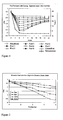
- the 12.7mm ID line was filled with a warm waxy crude oil and was cooled from a temperature of 45°C to 0°C over a period of 5.5 hours with the inlet valve closed and the outlet valve open.
- the open outlet was fitted with a vertical sight-tube as a riser.
- This riser initially contained approximately 30cm height of the waxy crude oil with the liquid level decreasing with cooling.
- the maximum hydrostatic head at the riser base was approximately 0.4 psig.
- the line was maintained at a constant temperature of 0°C for a further 24 hours, prior to re-starting flow. The results of this Example are shown in Figure 1 .
- Example 1 was repeated using the 5.9 mm ID line with both the inlet and outlet ports (0 and 8 respectively) open to atmosphere.
- the ends of the line were fitted with vertical sight-tubes as risers, initially containing approximately 30cm height of warm waxy crude.
- the liquid level in these tubes decreased with cooling.
- the maximum hydrostatic pressure at the start of cooling was approximately 0.4psig.
- the pressure gradients that developed are shown in Figure 3 .
- Example 2 was repeated with the 5.9mm ID horizontal line sealed by valves at both ends.
- Figure 4 shows that while significant sub-pressures developed with cooling, there was only a slight indication of pressure gradients along the line.
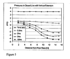
- the 5.9mm ID line was extended by a 3.3m vertical section, to provide a hydrostatic head at one end.
- the extended line [18.54m long] was loaded with waxy crude at a temperature of 45°C and both ends of the line were closed by valves.
- the vertical riser section was not enclosed with a coolant jacket. This vertical riser section produced approximately 3.9 psig hydrostatic pressure along the full 15.24 m horizontal section at time zero (when the valves were closed). A pronounced pressure gradient developed with cooling.
- a cavitation rig was constructed that comprises a flexible tube of 6.4 mm ID and 4.8 mm wall thickness with valves fitted at each end of the tube.
- the tube is formed into an inverted U shape and is arranged in a vertical plane with the ends of the tube in the same horizontal plane.
- the tube had a vertical rise of 1.4 metres.
- the viscous fracturing process was demonstrated using a simple rig comprising a flask having a lid wherein the lid has a borehole therethrough.
- a graduated 25 ml tube of 11.3 mm ID is inserted through the borehole of the lid in sealing engagement with the lid.
- a high-wax condensate (a fluid having a viscous resistance) is introduced into the flask and tube such that the fluid completely fills the flask and has a liquid level in the graduated 25 ml tube.
- the total fluid volume in the flask and tube is 660 ml.
- the rig (and hence the fluid) is then subjected to cooling.
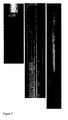
- the resultant fracturing is illustrated by the photographic images of Figure 7 .
- the gravity resistance shrinkage flow of the high-wax condensate is limited by its viscous resistance. Fracturing occurs even when a nitrogen gas pressure [10psig] was applied to the top of the graduated tube.
- a transparent model pipeline of 10m overall length was constructed to allow visualisation of test fluids.
- Five lengths of borosilicate glass tube, each having a length of 1.5m and an internal diameter (ID) of 6mm ID, and one length of borosilicate glass tube having a length of 0.5m and ID of 6mm were supported at their ends in machined acetal blocks.
- Each of these borosilicate glass tubes was arranged concentrically within a 100mm outer diameter (OD) clear extruded acrylic tube thereby creating cooling jackets for the borosilicate glass tubes.
- the blocks also supported the ends of the acrylic tubes.
- the concentrically arranged tubes were sealed into the end blocks with O-rings. Seven of the blocks were machined with ports for pressure transducers.
- the six glass tube sections were connected by flexible Tygon TM high pressure tubes of 6.4mm ID and 4.8mm wall thickness.
- the outer coolant chambers (formed by the annulus between the inner glass tube and outer acrylic tube) were each coupled with three parallel lengths of flexible reinforced PVC tube to minimise restriction of coolant flow.
- the flexible couplings were of variable length to allow a compact overall layout, and to allow the raising of individual sections to enable gravity assisted flow. These couplings were insulated with flexible padding.
- a waxy condensate was used in some tests and found to have too low a viscosity, when warm, to move the spheres reliably.
- An artificial variant of this fluid was prepared by adding 20% vol/vol of a high viscosity standard [N190000] to create a model fluid. Pour points of these fluids were determined as 24°C for the waxy condensate and 30°C for the model fluid [gelation points were approximately 21°C and 28°C respectively].
- the fluids were problematical because of their tendency to rapidly form extreme-viscosity, robust semi-solids, within a narrow temperature range. However, they had the advantage of being translucent and thus allowed the spheres to be easily seen. Their rapid onset gelation contributed to flow disruption and viscous fracturing.
- the sections of the transparent model pipeline were arranged in a horizontal configuration with one end of the pipeline closed and the other open to atmosphere. This approximated to the situation frequently used in laboratory restart test protocols.
- the model fluid described above was cooled from a temperature of 54°C to 18°C in 110 minutes. Three entrained spheres were observed and their movement recorded. The total movement of each sphere, is shown in Figure 8 , and clearly indicates a pattern of maximal flow at the open inlet with an approximately linear decrease in flow toward a shrinkage-null at the closed end. Pressure gradients along the line are shown in Figure 9 and display a gradient consistent with the flow direction.
- the sphere velocity can be calculated. If the sphere velocity, at its 1.2m locus, is assumed to be 0.88 of the maximum velocity, then a maximum velocity can be estimated for each temperature step. This is shown in Table 1 below. Although, the recorded pressure profiles are ragged, the line pressure-drops during each of these temperature steps can be extracted. By assuming that the average flow velocity in the full 10m length, during each step, is approximately half the maximum - as indicated by the movement of sphere B in Figure 8 , an approximate viscosity can be determined, consistent with the average flow and the measured pressure drop, for each of the four temperature steps. The calculated results are given in Table 2 below.
- the estimated viscosity values are surprisingly close to expected values for the model fluid, based on extrapolation from rheometry measurements and the values expected for a fluid at and below its measured pour point.
- the viscosity at a temperature of 40°C arises mainly from the 20% volume content of N190000 [N190000 viscosity at 40°C is 146.5Pas], while below the gelation temperature, the affect of wax formation predominates. Therefore, below a temperature of approximately 28°C, we might expect viscosities of approximately 1.0 x 10 3 Pas, and much higher as the temperature falls.
- the pressure increases towards the base of the raised section because of the hydrostatic head. This pressure is initially near constant along the horizontal section, and the pressure difference of approximately 2.7psi is consistent with the vertical rise and a density of approximately 800kg m -3 .
- a gradient develops from the riser base, owing to the shrinkage flow and increasing viscosity.
- Such a flow and pressure pattern is predicted by the model. No voids formed except at the raised end.
- a model field pipeline was compared with a model laboratory line.
- the model field pipeline had a length of 100km, a diameter of 1m and a gravity head (300 metre vertical rise) at one end [locus 0].
- the model field pipeline was sealed.
- the model laboratory line had a length of 15m, a diameter of 6mm diameter and a 0.5m sight-tube riser at one end [locus 0], which was open to atmosphere.
- the respective L/D ratios were 100,000 and 2,500, a 40-fold difference.
- both lines were subdivided into 12 equal-length sequential elements.
- the properties of the fluid, used in both lines, were based upon a waxy crude that has been extensively characterized.
- the temperature range and cooling rates were chosen to represent conditions that might be encountered with a land pipeline in temperate latitudes.
- the viscosity of the fluid at very low shear rates was determined by extrapolation from measured values.
- the fluid exhibited shear thinning behaviour that fitted closely to a power-law relationship under the measurement conditions. This relationship was determined at each of six temperatures covering the temperature range used for this model example. In a real-life study, it is recommended that viscosity is measured over the full shear rate range and a look-up table prepared for use with the model.
- shear-thinning fluids tend to exhibit more plug-like diametric flow-velocity profiles than the paraboloid form that typifies Newtonian pipe-flow.
- the near-wall velocity gradient is steeper and thus the true shear rate is higher than for the same volume flow-rate in Newtonian flow.
- the Weissenberg-Rabinowitsch correction is widely used to adjust laminar flow calculations where the sample exhibits shear thinning.
- the mean shear rate at the pipewall is found to be higher by a factor of approximately 1.9-fold in both field and model pipelines and the shear viscosity some 1.65-fold lower.
- the mean applied stress needed to maintain shrinkage-flow increases by approximately 1.15-fold.
- the fluid is assumed to become less shear thinning at shear rates below 0.01s -1 , then there is no change in calculation for the model field pipeline [minimum rate 0.0198s -1 ], but the viscosity estimates for the 15m model laboratory line are reduced.
- the estimated mean shear viscosity at the pipewall is reduced to approximately 723Pa. This is over 14-fold higher than the corrected viscosity estimate of approximately 51Pa for the 100km model filed pipeline.
- a distance/elevation map of a 300km section of pipeline having an internal diameter of 1m was processed to identify the way-points that affect the shrinkage flow, so as to reduce the computational requirement of the model.
- the effect of the first 25 hours of cooling is shown in Figure 20 .
- the initial fluid temperatures were close to 20°C at all points along the line.
- the temperatures along the pipeline, after 25 hours of cooling, were between 5°C and -2°C, depending mainly on pipeline elevation (above sea level).
- the fluid used for the model was a waxy crude that was rather more viscous than that used in Example 3.
- a viscosity / shear-rate matrix was built up from measured values for rates from 0.001s -1 to 600s -1 , at each of 36 temperature steps from minus 6°C to 29°C.
- the oil was markedly shear-thinning at all temperatures within this range of shear-rates.
- the maximum viscosity at the lowest shear-rate and temperature was 23,731Pa and the lowest viscosity at highest rate and temperature was 0.042Pa ⁇ s.
- Shrinkage flow was modelled on the basis of supplied liquid density data and supplied cooling projections for the line.
- the Weissenberg-Rabinowitsch correction was applied to the shear-rate calculation and viscosity changes were calculated from this adjusted rate, with reference to the supplied viscosity matrix.
- Hydrostatic pressures along the line were calculated from the elevation and density data. Flow equations were used to determine the pressure gradient needed to sustain shrinkage-flow. Void formation was assumed to occur at points where the pressure fell below minus 0.5barg.
- the fluid From the measured viscosity matrix, the fluid might have been expected to exhibit a viscosity of between 12,168Pa ⁇ at a temperature of 5 °C and 16,125Pa at a temperature of 2 °C, if shrinkage flow is not taken into account.
- the modelled viscosity values are far lower in most of the line sections with only the first short [10km] section exhibiting a very high value.
- the weighted mean viscosity for the full line length at 25 hours is predicted as about 191 Pa, some 70-fold lower than expected based upon rheometric measurement and little or no assumed shear.
- the void space development at the highest line point [67km] would probably be predicted by existing pipeline models, the additional voids indicated in Figure 20 are also likely to have a beneficial impact upon restart and early flow.
Landscapes
- Life Sciences & Earth Sciences (AREA)
- Engineering & Computer Science (AREA)
- Geology (AREA)
- Mining & Mineral Resources (AREA)
- Physics & Mathematics (AREA)
- Environmental & Geological Engineering (AREA)
- Fluid Mechanics (AREA)
- General Life Sciences & Earth Sciences (AREA)
- Geochemistry & Mineralogy (AREA)
- Pipeline Systems (AREA)
Abstract
A method of obtaining rheological data for a waxy fluid in a shut-in pipeline, the method comprising:
(A) creating a model of shrinkage flow in a shut-in pipeline by:
a) (i) determining the length and internal diameter of the pipeline, and (ii) obtaining a topographic relief map of the pipeline that identifies critical waypoints and entering the horizontal and vertical coordinates of these waypoints (relative to a selected low point) as model loci thereby creating a plurality of pipeline sub-sections;
b) calculating the hydrostatic pressure change across each pipeline sub-section;
c) determining the temperature profiles for a plurality of parameters of the waxy fluid over a temperature range typical of the temperatures encountered in the shut-in pipeline wherein the parameters include the density, shear stress, shear strain rate and vapour pressure of the waxy fluid;
d) entering a temperature change into the model for each pipeline subsection for a selected cooling time interval;
e) by reference to the density temperature profile, calculating the mean temperature in each pipeline sub-section, the volume change in each pipeline sub-section, and the resulting shrinkage flow rate in each pipeline sub-section;
f) by reference to the shrinkage flow rate in each pipeline subsection, the mean temperature in each pipeline sub-section, and the shear stress/shear strain rate temperature profile, calculating the wall shear strain rate in each sub-section, the shear viscosity in each sub-section and the pressure difference across each sub-section that is required to maintain shrinkage flow;
g) subtracting the required pressure difference across each sub-section from any existing pressure difference arising from a hydrostatic head and generating a pipeline pressure profile from the resultant pressure differences for the pipeline sub-sections;
h) if the line pressure at any locus fall below the vapour pressure of the waxy fluid at the locus temperature, a void is presumed to form at the locus and the fluid body in
i) the pipeline is divided at that locus; and
j) repeating steps (d) to (h) for a further cooling time interval; and
(B) using the model of shrinkage flow to (i) determine the distribution of any void spaces along the pipeline for the cooling time interval that the pipeline has been shut in; and, (ii) to obtain rheological data for the waxy fluid in each pipeline sub-section for the cooling time interval that the pipeline has been shut-in.
(A) creating a model of shrinkage flow in a shut-in pipeline by:
a) (i) determining the length and internal diameter of the pipeline, and (ii) obtaining a topographic relief map of the pipeline that identifies critical waypoints and entering the horizontal and vertical coordinates of these waypoints (relative to a selected low point) as model loci thereby creating a plurality of pipeline sub-sections;
b) calculating the hydrostatic pressure change across each pipeline sub-section;
c) determining the temperature profiles for a plurality of parameters of the waxy fluid over a temperature range typical of the temperatures encountered in the shut-in pipeline wherein the parameters include the density, shear stress, shear strain rate and vapour pressure of the waxy fluid;
d) entering a temperature change into the model for each pipeline subsection for a selected cooling time interval;
e) by reference to the density temperature profile, calculating the mean temperature in each pipeline sub-section, the volume change in each pipeline sub-section, and the resulting shrinkage flow rate in each pipeline sub-section;
f) by reference to the shrinkage flow rate in each pipeline subsection, the mean temperature in each pipeline sub-section, and the shear stress/shear strain rate temperature profile, calculating the wall shear strain rate in each sub-section, the shear viscosity in each sub-section and the pressure difference across each sub-section that is required to maintain shrinkage flow;
g) subtracting the required pressure difference across each sub-section from any existing pressure difference arising from a hydrostatic head and generating a pipeline pressure profile from the resultant pressure differences for the pipeline sub-sections;
h) if the line pressure at any locus fall below the vapour pressure of the waxy fluid at the locus temperature, a void is presumed to form at the locus and the fluid body in
i) the pipeline is divided at that locus; and
j) repeating steps (d) to (h) for a further cooling time interval; and
(B) using the model of shrinkage flow to (i) determine the distribution of any void spaces along the pipeline for the cooling time interval that the pipeline has been shut in; and, (ii) to obtain rheological data for the waxy fluid in each pipeline sub-section for the cooling time interval that the pipeline has been shut-in.
Description
- This invention relates to a method for determining the shear viscosity of a waxy crude oil or a waxy condensate in a pipeline when the pipeline has been shut-in under cold temperature conditions such that the oil or condensate cools down thereby forming a viscous liquid or gel that blocks the pipeline. In particular, the method of the present invention allows the shear viscosity of the waxy crude oil or waxy condensate to be determined in a plurality of sub-sections of the pipeline at one or more cooling time intervals.
- Pipelines are used in the oil industry for transporting crude oil or condensate from a separation facility (that separates gas and produced water from the crude oil or condensate) to either a refinery or an oil terminal. Such transportation pipelines may be on land or subsea and may be either buried in the ground/seabed or raised on stilts. In addition, waxy multiphase fluids may be transported from subsea wells through subsea flowlines (often referred to as subsea tie-backs) to a surface production facility via, for example, a riser.
- A problem may arise with pipelines that are used for transporting waxy crude oils (oils having a high proportion of waxy components) or waxy condensates when the pipeline is shut-in (for example, in an emergency or for routine maintenance). Thus, where the ambient temperature (external of the pipeline) is less than the bulk temperature of the crude oil in the pipeline, the bulk temperature of the crude oil or condensate may cool down to below the gelation temperature of the waxy fluid thereby forming a gel (a matrix of wax crystals in the oil or condensate) that blocks the pipeline. A similar problem may arise with subsea flowlines that are used for transporting waxy multiphase fluids when the subsea flowline is shut-in.
- The gel that forms on cooling a waxy crude oil, a waxy condensate or a waxy multiphase fluid is shear thinning (its viscosity decreases with flow) and starts to flow upon application of a sufficiently high pressure. Accordingly, a solution to the problem of re-starting flow through a gelled pipeline is to provide sufficient pressure to the gel to initiate flow. Traditionally, the re-start pressure for a gelled pipeline is determined using the following equation:

where L is the length of the pipeline;
τ is the yield stress of the gel; and
D is the internal diameter of the pipeline. - For a pipeline that is not provided with any pumping stations, the re-start pressure is applied at the separation facility where the oil or condensate enters the pipeline. For a pipeline that passes over land, pumping stations are generally provided at intervals along the pipeline. The re-start pressure is applied at the pumping station that is immediately before the shut-in (gelled) section of the pipeline. Accordingly, in the absence of a pumping station, the length, L, refers to the entire length of the pipeline. Where the
- pipeline has at least one pumping station, the length, L, refers to the distance between pumping stations, or the distance between the start of the pipeline and the first pumping station or the distance between the final pumping station and the end of the pipeline. The length, L, may be up to several hundreds of kilometres (km). Where the length, L, is relatively long, the pipeline operator may anticipate that flow could not be re-started if a gel forms in the pipeline owing to the calculated re-start pressure exceeding the maximum operating pressure of the pipeline. Accordingly, measures would need to be taken to mitigate the risk of forming a gel when the pipeline is shut-in. Such measures include:
- insulating the pipeline to prevent loss of heat from the crude oil or condensate to the external environment; heating the crude oil or condensate (for example, external heating of the pipeline); pumping hot crude oil or hot condensate down the pipeline such that the crude oil or condensate does not cool down to below its pour point upon shut-in of the pipeline; or the use of pour point depressants that lower the pour point temperature of the crude oil or condensate. However, these solutions are costly and may not be economic. It is also known that the re-start pressures that are predicted using the above equation may differ significantly from field experience. Thus, predicting the conditions necessary to restore flow in a gelled pipeline has long been recognised as a problem.
- It has now been found that when a pipeline is shut-in, the volume of a waxy fluid (for example, waxy crude oil or waxy condensate) decreases with cooling. For a given temperature change, the waxy fluid typically displays a greater degree of shrinkage than the material that comprises the pipeline, typically, steel. For a 10°C reduction in temperature, a waxy fluid such as a waxy crude oil or waxy condensate typically exhibits a shrinkage (net of steel pipe shrinkage) of at least 1% by volume. In a 100 km pipeline, this corresponds to 1 km of void space. If the waxy crude oil or waxy condensate is cooled slowly in a perfectly horizontal shut-in pipeline, the void space will form at the ends of the pipeline with the waxy fluid shrinking from both ends towards a shrinkage null point at approximately the halfway point in the pipeline. However, pipelines of significant length are not truly horizontal and will have high points and low points. Accordingly, where a topographical gradient exists that provides a vertical elevation for the pipeline that is greater than its internal diameter, shrinkage results in axially directed flow or flows toward the lowest point or points in the pipeline. Pressure gradients are induced by the shrinkage flow and become more pronounced as the viscosity of the waxy fluid increases with cooling. Thus, the pressure at any point in the pipeline is the combination of the hydrostatic pressure and the cohesive "tension" that causes the shrinkage. If the resultant (combined) pressure at a high point in the pipeline falls to below the vapour pressure of the waxy fluid, then a void is likely to form at the high point thereby dividing up the body of gelled or viscous fluid in the pipeline.
- As discussed above, the gel or viscous fluid that forms upon cooling a waxy fluid is shear-thinning. Accordingly, the shrinkage flow that arises upon cooling of a waxy fluid in a shut-in pipeline modifies the fluid/gel state of the waxy fluid, owing to viscous shearing. Also, where the fluid viscosity approaches the very high values typical of the laboratory measured pour points for waxy crude oils or waxy condensates, it may no longer be possible to sustain a flow rate sufficient to compensate the reduction in fluid volume that occurs with cooling. If this happens, the waxy fluid will tend to display fracture-void and/or bubble-void formation at locations in the pipeline where the pressure is below the vapour pressure of the waxy fluid. The fracture-voids tend to propagate in a substantially transverse direction (i.e. across the pipeline and not in a longitudinal direction). Fracturing of the fluid/gel continuum gives rise to discontinuities in the body of the fluid/gel, and these discontinuities effectively subdivide the fluid/gel into discrete lengths separated by vapour filled void spaces. It has now been found that the lower viscosity of the fluid/gel (arising from the shrinkage flow), and/or the distribution of void spaces at the high points in the pipeline, and/or the distribution of fracture-voids in the body of the fluid/gel may result in a significant reduction in the pressure required to re-start flow of the waxy fluid through the pipeline. Alternatively, the distribution of void spaces and intact fluid/gel may be used to identify sections of pipeline having the highest re-start pressure requirement such that a pipeline can be modified (either during the design stage or by modifying an existing pipeline) so as to reduce the re-start pressure.
- Thus, identification of the cavitation and flow processes induced by thermal shrinkage of a waxy fluid has allowed the construction of a mathematical model that predicts the distribution of fluid/gel viscosity and of vapour filled void-spaces within a gelled pipeline. This mathematical model allows the re-start pressure for a gelled shut-in pipeline to be determined, using a pipeline flow model, with greater accuracy than the prior art method discussed above.
- Thus, the present invention relates to a method of obtaining rheological data for a waxy fluid in a shut-in pipeline, the method comprising:
- (A) creating a model of shrinkage flow in a shut-in pipeline by:
- (a) (i) determining the length and internal diameter of the pipeline, and (ii) obtaining a topographic relief map of the pipeline that identifies critical waypoints and entering the horizontal and vertical coordinates of these waypoints (relative to a selected low point) as model loci thereby creating a plurality of pipeline sub-sections;
- (b) calculating the hydrostatic pressure change across each pipeline sub-section;
- (c) determining the temperature profiles for a plurality of parameters of the waxy fluid over a temperature range typical of the temperatures encountered in the shut-in pipeline wherein the parameters include the density, shear stress, shear strain rate and vapour pressure of the waxy fluid;
- (d) entering a temperature change into the model for each pipeline subsection for a selected cooling time interval;
- (e) by reference to the density temperature profile, calculating the mean temperature in each pipeline sub-section, the volume change in each pipeline sub-section, and the resulting shrinkage flow rate in each pipeline sub-section;
- (f) by reference to the shrinkage flow rate in each pipeline subsection, the mean temperature in each pipeline sub-section, and the shear stress/shear strain rate temperature profile, calculating the wall shear strain rate in each sub-section, the shear viscosity in each sub-section and the pressure difference across each sub-section that is required to maintain shrinkage flow;
- (g) subtracting the required pressure difference across each sub-section from any existing pressure difference arising from a hydrostatic head and generating a pipeline pressure profile from the resultant pressure differences for the pipeline sub-sections;
- (h) if the line pressure at any locus fall below the vapour pressure of the waxy fluid at the locus temperature, a void is presumed to form at the locus and the fluid body in the pipeline is divided at that locus; and
- (i) repeating steps (d) to (h) for a further cooling time interval; and (B) using the model of shrinkage flow to (i) determine the distribution of any void spaces along the pipeline for the cooling time interval that the pipeline has been shut in; and, (ii) to obtain rheological data for the waxy fluid in each pipeline sub-section for the cooling time interval that the pipeline has been shut-in.
- For avoidance of doubt, the term "pipeline" as used herein includes flowline.
- The rheological data generated by the model (wall shear strain rate and shear viscosity in each pipeline sub-section) may be inputted into a pipeline flow model for the more accurate prediction of the pressure required to re-start flow of fluid in the gelled pipeline and, optionally, the time required to re-start flow of fluid in the gelled pipeline. Suitable pipeline flow models are well known to the person skilled in the art and include OLGA 2000 marketed by Scandpower Petroleum Technology, the Stoner pipeline simulator (Stoner Software™) and the PipeSim™ model marketed by Schlumberger .
- Without wishing to be bound by any theory, it is also believed that the vapour filled void spaces at the high points in the pipeline and the vapour filled fracture-voids in the gelled sections of pipeline affect the rate at which the shear-thinning viscous liquid/gel breaks down during re-start of the flow through the pipeline. Thus, a shear-thinning liquid/gel may attain a higher velocity as it flows into a void space thereby reducing its viscosity. Accordingly, a pipeline flow model may be modified to take into account the presence of voids in the gelled pipeline thereby provided a more realistic prediction of the pressure required to re-start flow of fluid in the gelled pipeline, and, optionally, a more realistic prediction of the time required to re-start flow of fluid in the gelled pipeline.
- The pipeline model of the present invention is based on the following assumptions:
- 1. The pipeline is closed at both ends, for example, using valves or pumps. Where the pipeline is closed by a pump, the pump is not in operation and is therefore stationary.
- 2. The pipeline will follow the terrain of the land or seabed. Accordingly, the pipeline may have high points (or vertices) and low points.
- 3. When the bulk temperature of a waxy fluid (for example, a waxy crude oil or waxy condensate) is higher than the ambient temperature (external of the pipeline, the waxy fluid will cool when the pipeline is shut-in. There is a decrease in the volume of a waxy fluid with cooling (referred to herein as "thermal shrinkage"). Also, where the bulk temperature falls to below the critical gelation temperature, a gel will start to form in the pipeline.
- 4. Where the fluid body remains as an intact continuum, shrinkage flow must take place. This shrinkage flow is sustained by molecular cohesion forces within the waxy fluid.
- 5. Gravity influences this shrinkage flow. Thus, where a topographical gradient exists that provides a vertical elevation for the pipeline that is greater than its internal diameter, shrinkage results in axially directed flow or flows toward the lowest point or points in the pipeline.
- 6. The lowest point or points in the pipeline represent shrinkage nulls where flow ceases. The rate of flow increases with distance from the shrinkage nulls.
- 7. The rate of flow at any point in the pipeline depends upon the distance of that point from the shrinkage null, the rate of thermal change, the resultant fluid density change and the ratio of the length of the pipeline to the internal diameter of the pipeline [L/D ratio].
- 8. Pressure gradients are induced by the shrinkage flow and become more pronounced as the viscosity of the waxy fluid increases with cooling. Thus, the pressure at any point in the pipeline is the combination of the hydrostatic pressure and the cohesive "tension" that causes the shrinkage. If the resultant (combined) pressure at a high point in the pipeline falls to below the vapour pressure of the waxy fluid, then a void is likely to form at the high point.
- 9. If a pressure gradient can be sustained, either by a gravity-induced hydrostatic head or by applying pressure to the end of the pipeline, flow may continue in response to volume shrinkage. However, if the fluid viscosity approaches the very high values typical of the laboratory measured pour points for waxy crude oils or waxy condensates, then it may be no longer possible to sustain a flow rate sufficient to compensate the reduction in fluid volume. If this happens, the waxy fluid displays fracture and/or bubble void formation at locations in the pipeline where the pressure is below the vapour pressure of the waxy fluid. The fracture-voids tend to propagate in a substantially transverse direction (i.e. across the pipeline and not in a longitudinal direction). The resultant sub-division of the fluid body, alters the effective L/D ratio and thus reduces the flow rate required to compensate further shrinkage.
- 10. Multiple fracturing may occur thereby producing a plurality of short discrete lengths of gel.
- 11. The vapour pressure of the waxy crude oil or waxy condensate represents a finite lower limit of pressure, below which cohesive failure is likely.
- The following step protocol exemplifies the approach that may be used to develop the mathematical model of shrinkage flow in a pipeline:
- 1. Collect data for the field pipeline:
- Internal pipe diameter (and wall thickness if pressurised during shut-in);
- Line topographic relief (distance/height co-ordinates); and
- Line cooling profile during shut-in.
- 2. Collect data for the waxy fluid (waxy crude oil or waxy gas condensate):
- Density/temperature profile, over the temperature range relevant to the field conditions;
- Shear stress/shear strain rate profiles for shear rates from about 5s-1 to as low as possible, for a plurality of selected temperatures that fall within the temperature range relevant to the field conditions. Suitably, the selected temperatures are spaced apart over the entire temperature range; and
- 3. Collate the fluid property data in a form that is accessible for modelling purposes, such as look-up tables or formulaic relationships.
- 4. Simplify the line topographic relief map, for example, using an Excel™ macro to identify critical waypoints (slope reversals)
- 5. Enter the horizontal and vertical co-ordinates of these selected waypoints as model loci, thereby creating a plurality of pipeline sub-sections or elements (between adjacent loci, or between the start of the pipeline and the first locus or between the final locus and the end of the pipeline). The model then calculates the resultant hydrostatic pressure change across each element (using
Equation 1 below). - 6. Enter the element temperature changes for the first cooling time-step. By reference to the density/temperature relationship, the model calculates:
- The mean temperature in each element;
- the volume change (or shrinkage) in each element (from
Equations - the resultant shrinkage flow (using
Equations
- 7. From the calculated shrinkage flow rate in each element, the mean temperature in each element and the shear stress/shear strain rate profiles the following may be calculated:
- The wall shear strain rate [Weissenberg-Rabinowitsch corrected] in each element (using Equation 6);
- the shear viscosity in each element (using Equation 7); and
- the pressure difference (PD) required across each element (using Equation 8).
Accordingly, the present invention should be not be interpreted as being limited to the use of any specific rheological equations. - 8. The pressure difference, PD, across each element (that is required to maintain flow) is subtracted from any existing pressure difference that arises owing to the hydrostatic head.
- 9. The sequential element pressures are combined to provide a line pressure profile.
- 10. If the line pressure at any locus falls below the fluid vapour pressure (at that locus temperature) it is assumed that void formation occurs and the line is split at that locus for further computation.
- 11. Repeat the process from
step 6 for the next temperature change. - In practice, the first computation uses the full expected cooling range to provide a reasonable first approximation and to show whether or not any voids are likely to form. If voids are predicted, then a next best guess temperature fall is selected to focus in on the first appearance of a void.
- The equations used by this model example are set out below :

where zL is the vertical rise of the highest point in the line above an arbitrary datum,
z1 is the vertical rise of the locus of the first element in the flow direction (relative to the shrinkage null),
z2 is the vertical rise of the locus of the second element in the flow direction (relative to the shrinkage null) such that z2 is closer to the shrinkage null than is z1) g is the acceleration due to gravity, and ρ is the mean fluid density.
where ρ1 is the density at temperature T1,
and where ρ2 is the density at temperature T2.
where V1 is the element volume at T1,
and ΔT is the temperature change in that element.
The volume change in the steel pipe may be calculated separately and subtracted from the volume change of the hydrocarbon liquid to obtain a net liquid volume change, ΔVnet. Alternatively, the shrinkage coefficient for the steel pipe may be subtracted from that calculated for the hydrocarbon liquid to obtain ΔVnet directly.
where Σ ΔVnet is the sum of the volume changes in the element and in all the downstream elements toward the shrinkage null, and
t is the time duration of the cooling increment.
where A is the pipe cross-sectional area. - If the relationship between flow rate and flow resistance has been determined in the laboratory and that relationship has been expressed in terms of shear stress, σ, and shear strain rate γ, at each of a series of temperature steps such that for any selected temperature, a viscous consistency constant, K, and a shear thinning power index, n, may be derived, as in the expression σ=Kγn (at the temperature T), then:

v is the mean fluid velocity; and
r the internal pipe radius. - The shear viscosity η in each element is calculated from :

where K is the viscous consistency constant for the relationship between shear stress and shear strain rate at the mean element temperature (T1 + T2) / 2. - The pressure difference across each element, PD, that is needed to sustain the flow-rate, Q, is calculated from:

where L is the element length. - The above equation-set 6 to 8 assumes that the relationship between shear stress, σ, and shear strain rate, γ, has been accurately measured in the laboratory. For example, the shear stress, σ, may be determined with respect to the shear strain rate, by using rotational instruments (when the shear strain rate is known with acceptable accuracy [± 5%]) or by appropriate Weissenberg-Rabinowitsch correction of measurements made using tube viscometers. It is also assumed that a similar corrected rheological approach is applied to the pipeline flow model that predicts the pipeline re-start pressure and that shrinkage flow at the point of restart is allowed for.
- As discussed above, alternative rheological approaches may be used to determine the shear stress/shear strain rate temperature profile and to calculate the wall shear strain rate and shear viscosity in each pipeline sub-section. Accordingly, any assumptions that are used in determining these alternative rheological approaches should also be applied in the pipeline flow model that is used for determining the pipeline re-start pressure.
- The following model predictions are supported by experimental observations thereby validating the model:
- 1. Differential volume shrinkage between a pipe and a hydrocarbon liquid results in the formation of vapour-filled void-spaces during cooling.
- 2. Line pressure falls with cooling.
- 3. There is potential for void-space distribution at elevated vertices along the pipeline and the consequential subdivision of the liquid/gel column.
- 4. Fluid volume shrinkage may induce axially-directed, shear-inducing pipeline flow.
- 5. The maximal rate of shrinkage flow is directly proportional to the ratio of pipeline length and diameter
- 6. The viscous nature of the fluid/gel is altered by the rate of shrinkage flow.
- 7. Such flow may be influenced by stress applied by gravity or by an externally applied pressure, acting upon the shrinking fluid/gel.
- 8. Fracture-void formation may occur when the viscous flow-resistance of the fluid/gel, exceeds the available applied stress.
- The mathematical model may be used to predict the flow caused by thermal shrinkage at any locus along a pipeline and the consequent flow-induced pressure gradients. The model also predicts the effect of gravity in sustaining flow and supporting pressure gradients. In addition, the model predicts fluid/gel viscosity at any locus along the pipeline. The model also identifies the zones of fracture-void and bubble-void formation, where the applied stress caused by molecular adhesive forces and gravity is insufficient to maintain shrinkage-flow. If desired, a low pressure limit, below which fracture and/or bubble void formation is likely to occur within the fluid/gel column may be included in the model.
- The resultant map of changing viscosity and of void location along the pipeline, provides a far better guide to pipeline conditions prior to re-start, than is currently available. Such a map provides a basis for determining the requirements for successful re-start of flow of fluid through a pipeline. In particular, it has been found that cooling induced shrinkage flow can significantly reduce the viscosity of any gel that forms in a pipeline and may consequently lower the required re-start pressure for re-establishing flow through a pipeline.
- Varying the model parameters, allows investigation of different pipeline options including:
- 1. Pipeline dimensions and route.
- 2. Pumping station and valve location.
- 3. Effect of insulation of the pipeline or thermal variation.
- 4. Effect of shut-in duration.
- 5. Impact of changing fluid properties.
- 6. Effect of introducing artificial high points or vertices so as to assist shrinkage flow or induce void formation or both.
- 7. Changes in shut-in procedures.
Thus, the model may be used to optimise the design and route of the pipeline to aid the re-start of fluid flow in a gelled shut-in pipeline. The model may also be used to optimise shut-in procedures. - Advantages of the present invention include:
- 1) a reduction in the requirement to insulate the pipeline (rapid cooling of the waxy fluid may be beneficial to shrinkage flow);
- 2) a reduction in the amount or the elimination of the need for a pour point depressant (owing to a more realistic prediction of the shear viscosity of the waxy fluid under shut-in conditions);
- 3) a reduction in the predicted re-start pressure so that the pipeline can be re-started in cold conditions (where the bulk temperature of the crude oil or condensate has fallen to below its critical gelation temperature).
- The present invention also proposes designing a pipeline such that high points (vertices) are intentionally introduced to the pipeline. Accordingly, different pipeline routes over a particular terrain may be modelled such that a route may be selected that optimises shrinkage flow in the shut-in pipeline and/or optimizes the distribution of void spaces at the high points (vertices) in the pipeline. Optimisation of shrinkage flow in the pipeline may substantially reduce the re-start pressure for the shut-in pipeline owing to a reduction in the viscosity of the shear-thinning waxy fluid in the pipeline subsections.
- The model described above, may also be used to determine the optimum positioning of valves and/or pumps in the pipeline for maximising shrinkage flow and/or optimizing the distribution of void spaces at high points (vertices) in the pipeline. Thus, these valves and/or pumps may introduce artificial null points in the pipeline when a valve is closed (or is a non-return valve) or a pump is not being operated. The optimum positioning of the valves and/or pumps, as determined by the model, may be non-intuitive i.e. differ from established practice. For example, it is envisaged that non-return valves may be positioned in uphill portions of the pipeline, for example, approximately half way up a hill. Accordingly, the location in the pipeline immediately above a non-return valve, represents an artificial null point in the pipeline.
- The invention will now be described with reference to the following Figures and Examples.
- Two lines were constructed each having a length of 15.24m, one of 5.9mm internal diameter (ID) and the other of 12.7mm ID. Each line was formed into a horizontal double loop and was provided with an inlet and outlet valve. Both lines were enclosed by a common cooling jacket. Each line had ports located at its inlet and outlet and at intervals of 1.9 metres along the line with pressure transducers arranged at each port. Continuous logging of the pressure signals from the pressure transducers allowed investigation of pressure changes during the cooling phase and of pressure propagation events during restart. Provision was made for the addition of vertical sight tube risers at each end of the pipelines.
- The 12.7mm ID line, was filled with a warm waxy crude oil and was cooled from a temperature of 45°C to 0°C over a period of 5.5 hours with the inlet valve closed and the outlet valve open. The open outlet was fitted with a vertical sight-tube as a riser. This riser initially contained approximately 30cm height of the waxy crude oil with the liquid level decreasing with cooling. The maximum hydrostatic head at the riser base (prior to cooling) was approximately 0.4 psig. After cooling, the line was maintained at a constant temperature of 0°C for a further 24 hours, prior to re-starting flow. The results of this Example are shown in
Figure 1 . - It was found that pressure gradients developed with cooling resulting in a minimum (negative gauge pressure) at the closed end of the line and a maximum (atmospheric pressure) at the outlet. The minimum pressure was attained at the end of the cooling phase (when the temperature reached 0°C). The pressure gradients then decreased slowly during the subsequent low temperature soak period. However, pressures remained below atmospheric pressure at the point of re-starting flow through the line. These pressure gradients are shown in
Figure 2 at four time intervals (wherePort 0 is at the riser base). The pressure gradient results suggest a prolongation of flow events up to at least 24 hours after shut-in of a pipeline. - Example 1 was repeated using the 5.9 mm ID line with both the inlet and outlet ports (0 and 8 respectively) open to atmosphere. The ends of the line were fitted with vertical sight-tubes as risers, initially containing approximately 30cm height of warm waxy crude. The liquid level in these tubes decreased with cooling. The maximum hydrostatic pressure at the start of cooling was approximately 0.4psig. The pressure gradients that developed are shown in
Figure 3 . - Example 2 was repeated with the 5.9mm ID horizontal line sealed by valves at both ends.
Figure 4 shows that while significant sub-pressures developed with cooling, there was only a slight indication of pressure gradients along the line. - The 5.9mm ID line was extended by a 3.3m vertical section, to provide a hydrostatic head at one end. The extended line [18.54m long] was loaded with waxy crude at a temperature of 45°C and both ends of the line were closed by valves. The vertical riser section was not enclosed with a coolant jacket. This vertical riser section produced approximately 3.9 psig hydrostatic pressure along the full 15.24 m horizontal section at time zero (when the valves were closed). A pronounced pressure gradient developed with cooling.
- The results of this Example are shown in
Figure 5 . - A cavitation rig was constructed that comprises a flexible tube of 6.4 mm ID and 4.8 mm wall thickness with valves fitted at each end of the tube. The tube is formed into an inverted U shape and is arranged in a vertical plane with the ends of the tube in the same horizontal plane. The tube had a vertical rise of 1.4 metres.
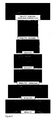
- If the highest point in the pipeline lies at an intermediate point along its length, then gravity tends to assist shrinkage flow in opposite directions, away from the high point vertex and toward shrinkage nulls at each end. In this situation, a void forms at the intermediate vertex. This may be demonstrated using the cavitation rig, described above. The tube of the cavitation rig was filled with a high-wax condensate, and the valves were then closed. Cooling of the tube resulted in a cavitation void forming at the apex of the tubing. A photographic sequence of the development of the void is shown in
Figure 6 . - The viscous fracturing process was demonstrated using a simple rig comprising a flask having a lid wherein the lid has a borehole therethrough. A graduated 25 ml tube of 11.3 mm ID is inserted through the borehole of the lid in sealing engagement with the lid. A high-wax condensate (a fluid having a viscous resistance) is introduced into the flask and tube such that the fluid completely fills the flask and has a liquid level in the graduated 25 ml tube. The total fluid volume in the flask and tube is 660 ml. The rig (and hence the fluid) is then subjected to cooling. The resultant fracturing is illustrated by the photographic images of
Figure 7 . Thus, the gravity resistance shrinkage flow of the high-wax condensate is limited by its viscous resistance. Fracturing occurs even when a nitrogen gas pressure [10psig] was applied to the top of the graduated tube. - A transparent model pipeline of 10m overall length was constructed to allow visualisation of test fluids. Five lengths of borosilicate glass tube, each having a length of 1.5m and an internal diameter (ID) of 6mm ID, and one length of borosilicate glass tube having a length of 0.5m and ID of 6mm were supported at their ends in machined acetal blocks. Each of these borosilicate glass tubes was arranged concentrically within a 100mm outer diameter (OD) clear extruded acrylic tube thereby creating cooling jackets for the borosilicate glass tubes. The blocks also supported the ends of the acrylic tubes. The concentrically arranged tubes were sealed into the end blocks with O-rings. Seven of the blocks were machined with ports for pressure transducers. The six glass tube sections were connected by flexible Tygon™ high pressure tubes of 6.4mm ID and 4.8mm wall thickness. The outer coolant chambers (formed by the annulus between the inner glass tube and outer acrylic tube) were each coupled with three parallel lengths of flexible reinforced PVC tube to minimise restriction of coolant flow. The flexible couplings were of variable length to allow a compact overall layout, and to allow the raising of individual sections to enable gravity assisted flow. These couplings were insulated with flexible padding.
- When loading this transparent model pipeline with test fluids, spherical plastic marker spheres were inserted to provide visual indication of cooling-induced flow events. The flow-patterns indicated by the movement of these spheres were broadly consistent with the model predictions. However, if the fluid approached the point of viscous fracture, then the flow patterns were necessarily disrupted.
- A waxy condensate was used in some tests and found to have too low a viscosity, when warm, to move the spheres reliably. An artificial variant of this fluid was prepared by adding 20% vol/vol of a high viscosity standard [N190000] to create a model fluid. Pour points of these fluids were determined as 24°C for the waxy condensate and 30°C for the model fluid [gelation points were approximately 21°C and 28°C respectively]. The fluids were problematical because of their tendency to rapidly form extreme-viscosity, robust semi-solids, within a narrow temperature range. However, they had the advantage of being translucent and thus allowed the spheres to be easily seen. Their rapid onset gelation contributed to flow disruption and viscous fracturing.
- The sections of the transparent model pipeline were arranged in a horizontal configuration with one end of the pipeline closed and the other open to atmosphere. This approximated to the situation frequently used in laboratory restart test protocols. For this test, the model fluid described above was cooled from a temperature of 54°C to 18°C in 110 minutes. Three entrained spheres were observed and their movement recorded. The total movement of each sphere, is shown in
Figure 8 , and clearly indicates a pattern of maximal flow at the open inlet with an approximately linear decrease in flow toward a shrinkage-null at the closed end. Pressure gradients along the line are shown inFigure 9 and display a gradient consistent with the flow direction. - By measuring the incremental movement of sphere A during each of four temperature steps, the sphere velocity can be calculated. If the sphere velocity, at its 1.2m locus, is assumed to be 0.88 of the maximum velocity, then a maximum velocity can be estimated for each temperature step. This is shown in Table 1 below. Although, the recorded pressure profiles are ragged, the line pressure-drops during each of these temperature steps can be extracted. By assuming that the average flow velocity in the full 10m length, during each step, is approximately half the maximum - as indicated by the movement of sphere B in
Figure 8 , an approximate viscosity can be determined, consistent with the average flow and the measured pressure drop, for each of the four temperature steps. The calculated results are given in Table 2 below. - Despite the high degree of approximation in the calculation, the estimated viscosity values are surprisingly close to expected values for the model fluid, based on extrapolation from rheometry measurements and the values expected for a fluid at and below its measured pour point. The viscosity at a temperature of 40°C arises mainly from the 20% volume content of N190000 [N190000 viscosity at 40°C is 146.5Pas], while below the gelation temperature, the affect of wax formation predominates. Therefore, below a temperature of approximately 28°C, we might expect viscosities of approximately 1.0 x 10³Pas, and much higher as the temperature falls.
- In this test, voids developed when the pressure had reached approximately -5psig.
Table 1 - Velocity Estimated from the Movement of Sphere A with Gelation Onset Observed at a Temperature of approximately 28°C. Time [mins] Temp [°C] Mean Step Temp [°C] Sphere Movement [mm] Sphere Velocity [m/s] Max Velocity [m/s] 0 54 57 29 41.5 141 4.12E-05 4.69E-05 75 24 26.5 6 1.33E-06 1.52E-06 92 20 22 3 5.43E-07 6.18E-07 110 18 19 2 3.03E-07 3.44E-07 Table 2 - Calculated viscosity Mean Step Temp [°C] Step Mean velocity [m/s] Estimated Viscosity [Pas] Estimated Pressure Difference [psig] Recorded psig 41.5 2.343 x 10⁻⁵ 13.1 0.41 0.41 26.5 7.56 x 10⁻⁷ 3,130 3.16 3.16 22 3.088 x 10⁻⁷ 11,800 4.86 4.86 19 1.722 x 10⁻⁷ 23,800 5.46 5.46 - Four of the sections of the transparent model pipeline were arranged in a horizontal configuration while a gravity-induced pressure head of 2.33m was created by raising two sections to form a vertical riser. Both ends of the line were closed. The model fluid was cooled from a temperature of 50°C to 25°C in 64 minutes. The movement of three entrained spheres indicates flow away from the raised end, decreasing toward a null at the other end. The movement of sphere A, shown in
Figure 10 , is far less than in the first example, partly because it is positioned at 3m rather than 1.2m as in the first example; and partly because of the reduced cooling range. The pressure profiles, shown inFigure 11 , were determined by the combined effect of the gravity head and shrinkage of the fluid with cooling. The lowest pressure was at the highest point where a void quickly forms. The pressure increases towards the base of the raised section because of the hydrostatic head. This pressure is initially near constant along the horizontal section, and the pressure difference of approximately 2.7psi is consistent with the vertical rise and a density of approximately 800kg m-3. When significant gel forms at a temperature below about 28°C, a gradient develops from the riser base, owing to the shrinkage flow and increasing viscosity. Such a flow and pressure pattern is predicted by the model. No voids formed except at the raised end. - In this test the sections of the transparent model flowline were arranged in a horizontal configuration and both ends of the flowline were open to atmosphere. This situation does not arise when a pipeline is shut in. In this test, a waxy condensate was cooled from a temperature of 38°C to 25°C in 100 minutes.
Figure 12 shows movement of sphere A that indicates flow away from its adjacent open end, but in this case, sphere C also indicates flow away from its adjacent open end [shown as a negative distance]. Thus there is bi-directional opposed flow toward a shrinkage-null near the mid-length, as also indicated by the limited movement of sphere B. The twin flow directions induce characteristic pressure profiles as shown inFigure 13 , with lowest pressures developing near the mid-length. Because cooling did not continue below the 21°C gelation temperature of the waxy condensate, there was limited pressure reduction and no fracture voids were formed. - In this test the sections of the transparent model flowline were arranged in a horizontal configuration and both ends of the line were closed. This is similar to certain laboratory test protocols. The model fluid was then cooled from 50°C to 15°C in 110 minutes. As in Example 3, there was bi-directional opposed flow, but far less than in Example 3.
Figure 17 shows that the flow pattern is markedly asymmetric with a shrinkage-null well to the right of the mid-length, probably because of the rig asymmetry. This very limited movement for such a wide temperature range is only possible if the flow is disrupted by fracturing to compensate for the shrinkage. Low pressures [seeFigure 18 ] and fractures [seeFigure 19 ], developed at an early stage during cooling. Pressure gradients were extremely limited. - To illustrate the potential value of the shrinkage model (described above), a model field pipeline was compared with a model laboratory line. For the purposes of clear comparison, conditions were chosen under which fracture-voids were not formed. The model field pipeline had a length of 100km, a diameter of 1m and a gravity head (300 metre vertical rise) at one end [locus 0]. The model field pipeline was sealed. The model laboratory line had a length of 15m, a diameter of 6mm diameter and a 0.5m sight-tube riser at one end [locus 0], which was open to atmosphere. The respective L/D ratios were 100,000 and 2,500, a 40-fold difference. For the model, both lines were subdivided into 12 equal-length sequential elements.
- The properties of the fluid, used in both lines, were based upon a waxy crude that has been extensively characterized. The temperature range and cooling rates were chosen to represent conditions that might be encountered with a land pipeline in temperate latitudes.
- The viscosity of the fluid at very low shear rates was determined by extrapolation from measured values. The fluid exhibited shear thinning behaviour that fitted closely to a power-law relationship under the measurement conditions. This relationship was determined at each of six temperatures covering the temperature range used for this model example. In a real-life study, it is recommended that viscosity is measured over the full shear rate range and a look-up table prepared for use with the model.
- The Tables below present a summary of the comparative modelling results. The calculations were repeated at four consecutive 5°C cooling steps, over a total 6 hours elapsed time. The fluid shrinkage is net of the steel pipe shrinkage.
Table 3 - Model prediction for a 100km pipeline cooled through 20°C in 6 hours Cooling Step [°C] 20 - 15 15 - 10 10 - 5 5 - 0 Elapsed Time [mins] 20 50 110 360 Cooling Rate [°C min-1] 0.25 0.175 0.083 0.02 Mean Velocity [ms-1] 0.199 0.132 0.063 0.016 Mean Shear Rate [s-1] 1.59 1.06 0.53 0.13 Mean Viscosity [Pas] 0.903 2.45 10.38 84.05 Linear Shrinkage [m] 477.8 475.3 472.8 470.3 Table 4 - Model prediction for the 15m laboratory rig cooled through 20°C in 6 hours Cooling Step [°C] 20 - 15 15 - 10 10 - 5 5 - 0 Elapsed Time [mins] 20 50 110 360 Cooling Rate [°C min-1] 0.25 0.175 0.083 0.02 Mean Velocity [ms-1] 3.0E-05 2.0E-05 9.8E-06 2.4E-06 Mean Shear Rate [s-1] 0.0398 0.0264 0.0131 0.0031 Mean Viscosity [Pas] 10.66 24.18 132.9 1,503 Linear Shrinkage [m] 0.0717 0.0713 0.0709 0.0706 - The linear distribution of line pressure and viscosity for the 100km pipeline are shown in
Figures 16 and18 respectively while the linear distribution of line pressure and viscosity for the 15 m laboratory line are shown inFigures 17 and19 respectively. The lowest line pressure in both cases is higher than the fluid vapour pressure at that temperature and it is thus assumed that no fracture voids formed. - Further support for model validity is gained by comparing the 15m rig model prediction of pressure distribution along the line, as in
Figure 17 , with the experimental results using a similar fluid, shown inFigure 2 . - It is observed that the fluid used for the model example, demonstrated a pour point of about 15°C [gel point of about 12°C], but the model indicates that there would be sufficient shear in the 15m rig to effectively delay this level of viscosity until the temperature falls to less than 5°C. In the 100km model comparison, the viscosity remained much lower at all stages.
- The model clearly indicates significant differences in viscosity development between the two pipelines. During the lowest temperature step the mean viscosity in the 15m line is nearly 18 times greater than in the 100km line. It would therefore be surprising if any subsequent laboratory estimation of restart pressure requirement were not pessimistic in such a case.
- For shear thinning liquids, the Weissenberg-Rabinowitsch correction is commonly used to adjust the calculation of the shear strain rate. Thus, shear-thinning fluids tend to exhibit more plug-like diametric flow-velocity profiles than the paraboloid form that typifies Newtonian pipe-flow. In consequence, the near-wall velocity gradient is steeper and thus the true shear rate is higher than for the same volume flow-rate in Newtonian flow.
- The Weissenberg-Rabinowitsch correction is widely used to adjust laminar flow calculations where the sample exhibits shear thinning. The pipewall shear strain rate, γw may thus be expressed as:

where n is the power law index derived from the relationship between shear stress and shear rate for that fluid, Q is the volume flow-rate, and r is the pipe radius. - If the power law index is known, then the shear viscosity at the pipewall under gravity flow, may be determined from:

where the velocity v is the mean value determined from the flow volume Q divided by the pipe cross-sectional area. - If there is significant shear thinning [n << 1], the shear viscosity near the wall is calculated to be much lower than in the Newtonian case [n = 1]. However, the shear rate in the main body of the fluid, will be far lower and the viscosity correspondingly higher.
- Applying such a shear rate correction to the last time step for the 100km model field pipeline and the 15m model laboratory line, the mean shear rate at the pipewall is found to be higher by a factor of approximately 1.9-fold in both field and model pipelines and the shear viscosity some 1.65-fold lower. Hence, the mean applied stress needed to maintain shrinkage-flow increases by approximately 1.15-fold.
- If in addition, the fluid is assumed to become less shear thinning at shear rates below 0.01s-1, then there is no change in calculation for the model field pipeline [minimum rate 0.0198s-1], but the viscosity estimates for the 15m model laboratory line are reduced. By assuming a gradual change in the power-law index, n, from 0.22 at 10-1s-1 to 0.3 at 5 x 10⁻⁴s-1, the estimated mean shear viscosity at the pipewall is reduced to approximately 723Pa. This is over 14-fold higher than the corrected viscosity estimate of approximately 51Pa for the 100km model filed pipeline.
- A distance/elevation map of a 300km section of pipeline having an internal diameter of 1m was processed to identify the way-points that affect the shrinkage flow, so as to reduce the computational requirement of the model. The effect of the first 25 hours of cooling is shown in
Figure 20 . The initial fluid temperatures were close to 20°C at all points along the line. The temperatures along the pipeline, after 25 hours of cooling, were between 5°C and -2°C, depending mainly on pipeline elevation (above sea level). The fluid used for the model was a waxy crude that was rather more viscous than that used in Example 3. - A viscosity / shear-rate matrix was built up from measured values for rates from 0.001s-1 to 600s-1, at each of 36 temperature steps from minus 6°C to 29°C. The oil was markedly shear-thinning at all temperatures within this range of shear-rates. The maximum viscosity at the lowest shear-rate and temperature was 23,731Pa and the lowest viscosity at highest rate and temperature was 0.042Pa·s.
- Shrinkage flow was modelled on the basis of supplied liquid density data and supplied cooling projections for the line. The Weissenberg-Rabinowitsch correction was applied to the shear-rate calculation and viscosity changes were calculated from this adjusted rate, with reference to the supplied viscosity matrix. Hydrostatic pressures along the line were calculated from the elevation and density data. Flow equations were used to determine the pressure gradient needed to sustain shrinkage-flow. Void formation was assumed to occur at points where the pressure fell below minus 0.5barg.
- It was assumed that pipeline pressure decreased rapidly on turn-down, so that a void formed at the 67 km high-point within 1 hour. From that time, shrinkage caused bi-directional flow away from this vertex. A second change in flow direction was predicted at 13 hours in the last line section [260km] and another at 18 hours when a void forms at the 252km high point. A final flow direction change was caused by a void forming at 20 hours at the 32 km high point. Voids were also predicted after 12 hours [10km] and at 18 hours [139km]. These voids changed flow velocity but not the flow direction. In all model calculations for this 25 hour cooling period, the predicted shear-rate was within the measured range of the supplied viscosity matrix. The resultant viscosity development is indicated by the boxed numbers [Pas], adjacent to relevant sections.
- From the measured viscosity matrix, the fluid might have been expected to exhibit a viscosity of between 12,168Pa·at a temperature of 5 °C and 16,125Pa at a temperature of 2 °C, if shrinkage flow is not taken into account. As shown in
Figure 20 , the modelled viscosity values are far lower in most of the line sections with only the first short [10km] section exhibiting a very high value. The weighted mean viscosity for the full line length at 25 hours is predicted as about 191 Pa, some 70-fold lower than expected based upon rheometric measurement and little or no assumed shear. In addition, while the void space development at the highest line point [67km] would probably be predicted by existing pipeline models, the additional voids indicated inFigure 20 are also likely to have a beneficial impact upon restart and early flow.
Claims (4)
- A method of obtaining rheological data for a waxy fluid in a shut-in pipeline, the method comprising:(A) creating a model of shrinkage flow in a shut-in pipeline by:(a) (i) determining the length and internal diameter of the pipeline, and (ii) obtaining a topographic relief map of the pipeline that identifies critical waypoints and entering the horizontal and vertical coordinates of these waypoints (relative to a selected low point) as model loci thereby creating a plurality of pipeline sub-sections;(b) calculating the hydrostatic pressure change across each pipeline sub-section;(c) determining the temperature profiles for a plurality of parameters of the waxy fluid over a temperature range typical of the temperatures encountered in the shut-in pipeline wherein the parameters include the density, shear stress, shear strain rate and vapour pressure of the waxy fluid;(d) entering a temperature change into the model for each pipeline subsection for a selected cooling time interval;(e) by reference to the density temperature profile, calculating the mean temperature in each pipeline sub-section, the volume change in each pipeline sub-section, and the resulting shrinkage flow rate in each pipeline sub-section;(f) by reference to the shrinkage flow rate in each pipeline subsection, the mean temperature in each pipeline sub-section, and the shear stress/shear strain rate temperature profile, calculating the wall shear strain rate in each sub-section, the shear viscosity in each sub-section and the pressure difference across each sub-section that is required to maintain shrinkage flow;(g) subtracting the required pressure difference across each sub-section from any existing pressure difference arising from a hydrostatic head and generating a pipeline pressure profile from the resultant pressure differences for the pipeline sub-sections;(h) if the line pressure at any locus fall below the vapour pressure of the waxy fluid at the locus temperature, a void is presumed to form at the locus and the fluid body in the pipeline is divided at that locus; and(i) repeating steps (d) to (h) for a further cooling time interval; and
B using the model of shrinkage flow to (i) determine the distribution of any void spaces along the pipeline for the cooling time interval that the pipeline has been shut in; and, (ii) to obtain rheological data for the waxy fluid in each pipeline sub-section for the cooling time interval that the pipeline has been shut-in. - A method of determining the pressure required to re-start flow of fluid through a gelled pipeline comprising:(A) creating a model of shrinkage flow in a shut-in pipeline by:(a) (i) determining the length and internal diameter of the pipeline, and (ii) obtaining a topographic relief map of the pipeline that identifies critical waypoints and entering the horizontal and vertical coordinates of these waypoints (relative to a selected low point) as model loci thereby creating a plurality of pipeline sub-sections;(b) calculating the hydrostatic pressure change across each pipeline sub-section;(c) determining the temperature profiles for a plurality of parameters of the waxy fluid over a temperature range typical of the temperatures encountered in the shut-in pipeline wherein the parameters include the density, shear stress, shear strain rate and vapour pressure of the waxy fluid;(d) entering a temperature change into the model for each pipeline subsection for a selected cooling time interval;(e) by reference to the density temperature profile, calculating the mean temperature in each pipeline sub-section, the volume change in each pipeline sub-section, and the resulting shrinkage flow rate in each pipeline sub-section;(f) by reference to the shrinkage flow rate in each pipeline subsection, the mean temperature in each pipeline sub-section, and the shear stress/shear strain rate temperature profile, calculating the wall shear strain rate in each sub-section, the shear viscosity in each sub-section and the pressure difference across each sub-section that is required to maintain shrinkage flow;(g) subtracting the required pressure difference across each sub-section from any existing pressure difference arising from a hydrostatic head and generating a pipeline pressure profile from the resultant pressure differences for the pipeline sub-sections;(h) if the line pressure at any locus fall below the vapour pressure of the waxy fluid at the locus temperature, a void is presumed to form at the locus and the fluid body inthe pipeline is divided at that locus; and
(i) repeating steps (d) to (h) for a further cooling time interval; and(B) using the model of shrinkage flow to obtain rheological data for the waxy fluid in each pipeline sub-section for the cooling time interval that the pipeline has been shut-in; and(C) inputting the rheological data obtained in step (B) into a pipeline flow model and using the pipeline flow model to predict the pressure required to re-start flow of fluid through the pipeline. - A method of determining a pipeline route comprising:(A) identifying a plurality of potential pipeline routes over a terrain;(B) creating models as defined in Claim 1 for each of the potential pipeline routes;(C) selecting the model and hence the pipeline route that maximizes fluid volume shrinkage.
- A method of determining the optimal location of valves and/or pumps in a pipeline comprising:(A) creating a model for a pipeline using the method defined in Claim 1 wherein the horizontal and vertical coordinates of valves and/or pumps along the pipeline are entered into the model as additional model loci; and(B) creating at least one further model, preferably, a plurality of further models, for the pipeline wherein the locations of the valves and/or pumps along the pipeline are varied; and(C) selecting the model and hence the location of the valves and/or pumps that maximises fluid volume shrinkage.
Priority Applications (2)
| Application Number | Priority Date | Filing Date | Title |
|---|---|---|---|
| EP08250474A EP2088281A1 (en) | 2008-02-08 | 2008-02-08 | Method for determining the viscosity of a waxy fluid in a shut-in pipeline |
| PCT/GB2009/000293 WO2009098447A2 (en) | 2008-02-08 | 2009-02-04 | Method for determining the viscosity of a waxy fluid in a shut-in pipeline |
Applications Claiming Priority (1)
| Application Number | Priority Date | Filing Date | Title |
|---|---|---|---|
| EP08250474A EP2088281A1 (en) | 2008-02-08 | 2008-02-08 | Method for determining the viscosity of a waxy fluid in a shut-in pipeline |
Publications (1)
| Publication Number | Publication Date |
|---|---|
| EP2088281A1 true EP2088281A1 (en) | 2009-08-12 |
Family
ID=39672953
Family Applications (1)
| Application Number | Title | Priority Date | Filing Date |
|---|---|---|---|
| EP08250474A Ceased EP2088281A1 (en) | 2008-02-08 | 2008-02-08 | Method for determining the viscosity of a waxy fluid in a shut-in pipeline |
Country Status (1)
| Country | Link |
|---|---|
| EP (1) | EP2088281A1 (en) |
Cited By (4)
| Publication number | Priority date | Publication date | Assignee | Title |
|---|---|---|---|---|
| FR2976670A1 (en) * | 2011-06-17 | 2012-12-21 | IFP Energies Nouvelles | Method for estimating restarting conditions of paraffinic hydrocarbon flow in pipe utilized to transport hydrocarbons to oil field, involves simulating restart phase, and evaluating value of pressure re-circulating hydrocarbon in pipe |
| CN112012728A (en) * | 2020-08-19 | 2020-12-01 | 中国石油天然气股份有限公司 | Method for determining flow velocity of polymer in reservoir interstitial space |
| CN113916747A (en) * | 2021-10-14 | 2022-01-11 | 重庆科技学院 | Revision method applied to viscoelastic fluid test starting pressure gradient |
| CN115405863A (en) * | 2022-07-28 | 2022-11-29 | 国家管网集团北方管道有限责任公司 | Intelligent scheduling control system and method for oil pipeline |
Citations (2)
| Publication number | Priority date | Publication date | Assignee | Title |
|---|---|---|---|---|
| US3780751A (en) * | 1972-12-04 | 1973-12-25 | Atlantic Richfield Co | Restoring oil flow in a pipeline |
| US3791395A (en) * | 1972-12-15 | 1974-02-12 | Atlantic Richfield Co | Restarting flow of gelled oil |
-
2008
- 2008-02-08 EP EP08250474A patent/EP2088281A1/en not_active Ceased
Patent Citations (2)
| Publication number | Priority date | Publication date | Assignee | Title |
|---|---|---|---|---|
| US3780751A (en) * | 1972-12-04 | 1973-12-25 | Atlantic Richfield Co | Restoring oil flow in a pipeline |
| US3791395A (en) * | 1972-12-15 | 1974-02-12 | Atlantic Richfield Co | Restarting flow of gelled oil |
Non-Patent Citations (4)
| Title |
|---|
| DAVIDSON M R ET AL: "A model for restart of a pipeline with compressible gelled waxy crude oil", JOURNAL OF NON-NEWTONIAN FLUID MECHANICS, ELSEVIER, NL, vol. 123, no. 2-3, 10 November 2004 (2004-11-10), pages 269 - 280, XP004650585, ISSN: 0377-0257 * |
| FRIGAARD I ET AL: "Compressible displacement of waxy crude oils in long pipeline startup flows", JOURNAL OF NON-NEWTONIAN FLUID MECHANICS, ELSEVIER, NL, vol. 147, no. 1-2, 15 November 2007 (2007-11-15), pages 45 - 64, XP008095351, ISSN: 0377-0257 * |
| LU TAO, JIANG PEX-XUE: "Heat transfer model and numerical simulation of temperature decreasing and oil solidifying of buried crude pipeline during shutdown", JOURNAL OF THERMAL SCIENCE AND TECHNOLOGY, vol. 4, 31 December 2005 (2005-12-31), pages 298 - 302, XP008095474 * |
| VINAY ET AL: "Numerical simulation of weakly compressible Bingham flows: The restart of pipeline flows of waxy crude oils", JOURNAL OF NON-NEWTONIAN FLUID MECHANICS, ELSEVIER, NL, vol. 136, no. 2-3, 15 July 2006 (2006-07-15), pages 93 - 105, XP005494025, ISSN: 0377-0257 * |
Cited By (7)
| Publication number | Priority date | Publication date | Assignee | Title |
|---|---|---|---|---|
| FR2976670A1 (en) * | 2011-06-17 | 2012-12-21 | IFP Energies Nouvelles | Method for estimating restarting conditions of paraffinic hydrocarbon flow in pipe utilized to transport hydrocarbons to oil field, involves simulating restart phase, and evaluating value of pressure re-circulating hydrocarbon in pipe |
| CN112012728A (en) * | 2020-08-19 | 2020-12-01 | 中国石油天然气股份有限公司 | Method for determining flow velocity of polymer in reservoir interstitial space |
| CN112012728B (en) * | 2020-08-19 | 2024-03-26 | 中国石油天然气股份有限公司 | Method for determining flow velocity of polymer between reservoir gaps |
| CN113916747A (en) * | 2021-10-14 | 2022-01-11 | 重庆科技学院 | Revision method applied to viscoelastic fluid test starting pressure gradient |
| CN113916747B (en) * | 2021-10-14 | 2023-09-15 | 重庆科技学院 | A revised method for testing activation pressure gradients applied to viscoelastic fluids |
| CN115405863A (en) * | 2022-07-28 | 2022-11-29 | 国家管网集团北方管道有限责任公司 | Intelligent scheduling control system and method for oil pipeline |
| CN115405863B (en) * | 2022-07-28 | 2023-09-01 | 国家管网集团北方管道有限责任公司 | An intelligent scheduling control system and method for oil pipelines |
Similar Documents
| Publication | Publication Date | Title |
|---|---|---|
| US4726219A (en) | Method and system for determining fluid pressures in wellbores and tubular conduits | |
| US8973433B2 (en) | Dual differential pressure multiphase flow meter | |
| CN103590818B (en) | Method and device for semi-analytical determination of temperature distribution in wellbore | |
| Mukherjee et al. | Experimental study of oil-water flow in inclined pipes | |
| Shi | A study on high-viscosity oil-water two-phase flow in horizontal pipes | |
| Xu | Analysis of diagnostic testing of sustained casing pressure in wells | |
| US20180245463A1 (en) | Method for determining a water cut of an oil-water mixture produced from an oil well | |
| WO2009098447A2 (en) | Method for determining the viscosity of a waxy fluid in a shut-in pipeline | |
| Ihara et al. | Experimental and theoretical investigation of two-phase flow in horizontal wells | |
| Phillips et al. | Novel approaches to waxy crude restart: Part 2: An investigation of flow events following shut down | |
| Pourafshary | A coupled wellbore/reservoir simulator to model multiphase flow and temperature distribution | |
| US7240537B2 (en) | Method for the determination of the wall friction profile along pipes by pressure transients measurements | |
| Xu et al. | Trapped water flushed by flowing oil in upward-inclined oil pipelines | |
| Zhang et al. | Simulation Studies of Wax Deposition in Oil-Gas Inclined Shafte | |
| Ualiyeva et al. | Experimental Characterization of Gas-Liquid Downward Flow | |
| RU2803086C1 (en) | Method for eliminating a gas blowout in wells in offshore conditions | |
| An et al. | Estimation of bottomhole pressure in pumping oil wells: effect of high-viscosity fluids and casinghead pressure | |
| US20240209849A1 (en) | Method for simulating the effect of plugs on cement placement | |
| Gould et al. | Design of Offshore Gas Pipelines Accounting For Two-Phase Flow (includes associated papers 6401 and 6402) | |
| Wang | Experiments and model development for high-viscosity oil/water/gas horizontal and upward vertical pipe flows | |
| Ömürlü | Mathematical modeling of horizontal two-phase flow through fully eccentric annuli | |
| Croce et al. | Mechanistic Model for the Design and Operation of an Intermittent Gas Lift System for Liquid Loaded Horizontal Gas Wells | |
| CN111581584B (en) | Quantitative calculation method for pressure drop heat exchange in geothermal development process | |
| Wordu et al. | A Study of Pressure Gradient in Multiphase Flow in Vertical Pipes | |
| Williams et al. | Measurement of break away yield stress of waxy crude oil and pipeline restart system design |
Legal Events
| Date | Code | Title | Description |
|---|---|---|---|
| PUAI | Public reference made under article 153(3) epc to a published international application that has entered the european phase |
Free format text: ORIGINAL CODE: 0009012 |
|
| AK | Designated contracting states |
Kind code of ref document: A1 Designated state(s): AT BE BG CH CY CZ DE DK EE ES FI FR GB GR HR HU IE IS IT LI LT LU LV MC MT NL NO PL PT RO SE SI SK TR |
|
| AX | Request for extension of the european patent |
Extension state: AL BA MK RS |
|
| STAA | Information on the status of an ep patent application or granted ep patent |
Free format text: STATUS: THE APPLICATION HAS BEEN REFUSED |
|
| 18R | Application refused |
Effective date: 20090912 |