EP1801706A2 - PCR elbow determination by use of a double sigmoid function curve fit with the Levenberg-Marquardt algorithm and normalization - Google Patents
PCR elbow determination by use of a double sigmoid function curve fit with the Levenberg-Marquardt algorithm and normalization Download PDFInfo
- Publication number
- EP1801706A2 EP1801706A2 EP06026118A EP06026118A EP1801706A2 EP 1801706 A2 EP1801706 A2 EP 1801706A2 EP 06026118 A EP06026118 A EP 06026118A EP 06026118 A EP06026118 A EP 06026118A EP 1801706 A2 EP1801706 A2 EP 1801706A2
- Authority
- EP
- European Patent Office
- Prior art keywords
- curve
- parameters
- value
- normalized
- dataset
- Prior art date
- Legal status (The legal status is an assumption and is not a legal conclusion. Google has not performed a legal analysis and makes no representation as to the accuracy of the status listed.)
- Granted
Links
Images






Classifications
-
- G—PHYSICS
- G06—COMPUTING OR CALCULATING; COUNTING
- G06F—ELECTRIC DIGITAL DATA PROCESSING
- G06F17/00—Digital computing or data processing equipment or methods, specially adapted for specific functions
- G06F17/10—Complex mathematical operations
-
- G—PHYSICS
- G06—COMPUTING OR CALCULATING; COUNTING
- G06F—ELECTRIC DIGITAL DATA PROCESSING
- G06F17/00—Digital computing or data processing equipment or methods, specially adapted for specific functions
- G06F17/10—Complex mathematical operations
- G06F17/17—Function evaluation by approximation methods, e.g. inter- or extrapolation, smoothing, least mean square method
-
- C—CHEMISTRY; METALLURGY
- C12—BIOCHEMISTRY; BEER; SPIRITS; WINE; VINEGAR; MICROBIOLOGY; ENZYMOLOGY; MUTATION OR GENETIC ENGINEERING
- C12Q—MEASURING OR TESTING PROCESSES INVOLVING ENZYMES, NUCLEIC ACIDS OR MICROORGANISMS; COMPOSITIONS OR TEST PAPERS THEREFOR; PROCESSES OF PREPARING SUCH COMPOSITIONS; CONDITION-RESPONSIVE CONTROL IN MICROBIOLOGICAL OR ENZYMOLOGICAL PROCESSES
- C12Q1/00—Measuring or testing processes involving enzymes, nucleic acids or microorganisms; Compositions therefor; Processes of preparing such compositions
- C12Q1/68—Measuring or testing processes involving enzymes, nucleic acids or microorganisms; Compositions therefor; Processes of preparing such compositions involving nucleic acids
- C12Q1/6844—Nucleic acid amplification reactions
- C12Q1/6851—Quantitative amplification
-
- G—PHYSICS
- G06—COMPUTING OR CALCULATING; COUNTING
- G06F—ELECTRIC DIGITAL DATA PROCESSING
- G06F2218/00—Aspects of pattern recognition specially adapted for signal processing
- G06F2218/02—Preprocessing
-
- G—PHYSICS
- G06—COMPUTING OR CALCULATING; COUNTING
- G06F—ELECTRIC DIGITAL DATA PROCESSING
- G06F2218/00—Aspects of pattern recognition specially adapted for signal processing
- G06F2218/08—Feature extraction
- G06F2218/10—Feature extraction by analysing the shape of a waveform, e.g. extracting parameters relating to peaks
Definitions
- the present invention relates generally to systems and methods for processing data representing sigmoid or growth curves, and more particularly to systems and methods for determining characteristic cycle threshold (Ct) or elbow values in PCR amplification curves.
- Ct characteristic cycle threshold
- PCR Polymerase Chain Reaction
- the Polymerase Chain Reaction is an in vitro method for enzymatically synthesizing or amplifying defined nucleic acid sequences.
- the reaction typically uses two oligonucleotide primers that hybridize to opposite strands and flank a template or target DNA sequence that is to be amplified. Elongation of the primers is catalyzed by a heat-stable DNA polymerase. A repetitive series of cycles involving template denaturation, primer annealing, and extension of the annealed primers by the polymerase results in an exponential accumulation of a specific DNA fragment.
- Fluorescent probes or markers are typically used in the process to facilitate detection and quantification of the amplification process.
- thermocyclers which include components and devices for measuring fluorescence signals during the amplification reaction.
- An example of such a thermocycler is the Roche Diagnostics LightCycler (Cat. No. 20110468).
- the amplification products are, for example, detected by means of fluorescent labeled hybridization probes which only emit fluorescence signals when they are bound to the target nucleic acid or in certain cases also by means of fluorescent dyes that bind to double-stranded DNA.
- identifying a transition point at the end of the baseline region which is referred to commonly as the elbow value or cycle threshold (Ct) value, is extremely useful for understanding characteristics of the PCR amplification process.
- the Ct value may be used as a measure of efficiency of the PCR process. For example, typically a defined signal threshold is determined for all reactions to be analyzed and the number of cycles (Ct) required to reach this threshold value is determined for the target nucleic acid as well as for reference nucleic acids such as a standard or housekeeping gene.
- the absolute or relative copy numbers of the target molecule can be determined on the basis of the Ct values obtained for the target nucleic acid and the reference nucleic acid ( Gibson et al., Genome Research 6:995-1001 ; Bieche et al., Cancer Research 59:2759-2765, 1999 ; WO 97/46707 ; WO 97/46712 ; WO 97/46714 ).
- the elbow value (20) at the end of the baseline region (15) in FIG. 1 would be in the region of cycle number 30.
- the elbow value in a PCR curve can be determined using several existing methods. For example, various current methods determine the actual value of the elbow as the value where the fluorescence reaches a predetermined level called the AFL (arbitrary fluorescence value). Other current methods might use the cycle number where the second derivative of fluorescence vs. cycle number reaches a maximum. All of these methods have severe drawbacks. For example, some methods are very sensitive to outlier (noisy) data, and the AFL value approach does not work well for data sets with high baselines. Traditional methods to determine the baseline stop (or end of the baseline) for the growth curve shown in FIG. 1 may not work satisfactorily, especially in a high titer situation. Furthermore, these algorithms typically have many parameters (e.g., 50 or more) that are poorly defined, linearly dependent, and often very difficult, if not impossible, to optimize.
- parameters e.g., 50 or more
- the present invention provides novel, efficient systems and methods for determining characteristic transition values such as elbow values in sigmoid or growth-type curves.
- the systems and methods of the present invention are particularly useful for determining the cycle threshold (Ct) value in PCR amplification curves.
- a double sigmoid function with parameters determined by a Levenberg-Marquardt (LM) regression process is used to find an approximation to a curve that fits a PCR dataset.
- the curve can be normalized using one or more of the determined parameters. Normalization is advantageous for determining the Ct value if one chooses the arbitrary fluorescence level (AFL) approach to calculating Ct values for amplification curves.
- AFL arbitrary fluorescence level
- the normalized curve is processed by applying a root-finding algorithm to determine the root of the function representing the normalized curve, which root corresponds to the Ct value. The Ct value is then returned and may be displayed or otherwise used for further processing.
- a computer implemented method of determining a point at the end of the baseline region of a growth curve comprising the steps of:
- a computer-readable medium including code for controlling a processor to determine a point at the end of the baseline region of a growth curve is provided, wherein the code includs instructions to:
- PCR kinetic Polymerase Chain Reaction
- the present invention provides systems and methods for determining a transition value in a sigmoid or growth curve, such as the end of the baseline region or the elbow value or Ct value of a kinetic PCR amplification curve.
- a double sigmoid function with parameters determined by a Levenberg-Marquardt (LM) regression process is used to find an approximation to the curve.
- the curve can be normalized using one or more of the determined parameters. Normalization is advantageous for determining the Ct value if one chooses the arbitrary fluorescence level (AFL) approach to calculating Ct values for amplification curves.
- AFL arbitrary fluorescence level
- the normalized curve is processed by applying a root-finding algorithm to determine the root of the function representing the normalized curve, which root corresponds to the Ct value.
- the Ct value is then returned and may be displayed or otherwise used for further processing.
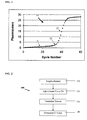
- FIG. 1 One example of an amplification curve 10 in the context of a PCR process is shown in FIG. 1.
- the curve 10 includes a lag phase region 15, and an exponential phase region 25.
- Lag phase region 15 is commonly referred to as the baseline or baseline region.
- Such a curve 10 includes a transitionary region of interest 20 linking the lag phase and the exponential phase regions.
- Region 20 is commonly referred to as the elbow or elbow region.
- the elbow region typically defines an end to the baseline and a transition in the growth or amplification rate of the underlying process.
- Identifying a specific transition point in region 20 can be useful for analyzing the behavior of the underlying process.
- identifying a transition point referred to as the elbow value or cycle threshold (Ct) value is extremely useful for understanding efficiency characteristics of the PCR process.
- SDA strand displacement amplification
- NASBA nucleic acid sequence-based amplification
- TMA transcription mediated amplification
- data for a typical PCR growth curve can be represented in a two-dimensional coordinate system, for example, with PCR cycle number defining the x-axis and an indicator of accumulated polynucleotide growth defining the y-axis.
- the indicator of accumulated growth is a fluorescence intensity value as the use of fluorescent markers is perhaps the most widely used labeling scheme. However, it should be understood that other indicators may be used depending on the particular labeling and/or detection scheme used.
- Examples of other useful indicators of accumulated signal growth include luminescence intensity, chemiluminescence intensity, bioluminescence intensity, phosphorescence intensity, charge transfer, voltage, current, power, energy, temperature, viscosity, light scatter, radioactive intensity, reflectivity, transmittance and absorbance.
- the definition of cycle can also include time, process cycles, unit operation cycles and reproductive cycles.
- step 110 an experimental data set representing the curve is received or otherwise acquired.
- An example of a plotted PCR data set is shown in FIG. 1, where the y-axis and x-axis represent fluorescence intensity and cycle number, respectively, for a PCR curve.
- the data set should include data that is continuous and equally spaced along an axis.
- the method may be implemented by using conventional personal computer systems including, but not limited to, an input device to input a data set, such as a keyboard, mouse, and the like; a display device to represent a specific point of interest in a region of a curve, such as a monitor; a processing device necessary to carry out each step in the method, such as a CPU; a network interface such as a modem a data storage device to store the data set, a computer code running on the processor and the like.
- the method may also be implemented in a PCR device.
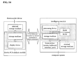
- FIG. 14 shows a general block diagram explaining the relation between the software and hardware resources.
- the system comprises a kinetic PCR analysis module which may be located in a thermocycler device and an intelligence module which is part of the computer system.
- the data sets (PCR data sets) are transferred from the analysis module to the intelligence module or vice versa via a network connection or a direct connection.
- the data sets are processed according to the method as displayed in Fig. 2 by computer code running on the processor and being stored on the storage device of the intelligence module and after processing transferred back to the storage device of the analysis module, where the modified data may be displayed on a displaying device.
- the intelligence module may also be implemented in the PCR data acquiring device.
- the data set may be provided to the intelligence module in real time as the data is being collected, or it may be stored in a memory unit or buffer and provided to the intelligence module after the experiment has been completed.
- the data set may be provided to a separate system such as a desktop computer system or other computer system, via a network connection (e.g., LAN, VPN, intranet, Internet, etc.) or direct connection (e.g., USB or other direct wired or wireless connection) to the acquiring device, or provided on a portable medium such as a CD, DVD, floppy disk or the like.
- a network connection e.g., LAN, VPN, intranet, Internet, etc.
- direct connection e.g., USB or other direct wired or wireless connection
- the data set includes data points having a pair of coordinate values (or a 2-dimensional vector).
- the pair of coordinate values typically represents the cycle number and the fluorescence intensity value.
- step 120 an approximation of the curve is calculated.
- a double sigmoid function with parameters determined by a Levenberg-Marquardt (LM) regression process or other regression process is used to find an approximation of a curve representing the data set.
- the approximation is said to be "robust" as outlier or spike points have a minimal effect on the quality of the curve fit.
- FIG 2 illustrates a plot of the received data set and a robust approximation of the data set determined by using a Levenberg-Marquardt regression process to determine the parameters of a double sigmoid function according to the present invention.
- outlier or spike points in the dataset are removed or replaced prior to processing the data set to determine the end of the baseline region.
- Spike a removal may occur before or after the dataset is acquired in step 110.
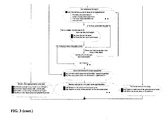
- FIG. 3 illustrates the process flow for identifying and replacing spike points in datasets representing PCR or other growth curves.
- step 130 the parameters determined in step 120 are used to normalize the curve, as will be described in more detail below. Normalization in this manner allows for determining the Ct value without having to determine or specify the end of the baseline region of the curve or a baseline stop position.
- step 140 the normalized curve is then processed to determine the Ct value as will be discussed in more detail below.
- Steps 502 through 524 of FIG. 3 also illustrate a process flow for approximating the curve of a dataset and determining the parameters of a fit function (step 120). These parameters can be used in normalizing the curve, e.g., modifying or removing the baseline slope of the data set representing a sigmoid or growth type curve such as a PCR curve according to one embodiment of the present invention (step 130). Where the dataset has been processed to produce a modified dataset with removed or replaced spike points, the modified spikeless dataset may be processed according to steps 502 through 524 to identify the parameters of the fit function.
- a Levenberg-Marquardt (LM) method is used to calculate a robust curve approximation of a data set.
- the LM method is a non-linear regression process; it is an iterative technique that minimizes the distance between a non-linear function and a data set.
- the process behaves like a combination of a steepest descent process and a Gauss-Newton process: when the current approximation doesn't fit well it behaves like the steepest descent process (slower but more reliable convergence), but as the current approximation becomes more accurate it will then behave like the Gauss-Newton process (faster but less reliable convergence).
- the LM regression method is widely used to solve non-linear regression problems.
- the LM regression method includes an algorithm that requires various inputs and provides output.
- the inputs include a data set to be processed, a function that is used to fit the data, and an initial guess for the parameters or variables of the function.
- the output includes a set of parameters for the function that minimizes the distance between the function and the data set.
- the double sigmoid equation (1) has 7 parameters: a, b, c, d, e, f and g.
- the equation can be decomposed into a sum of a constant, a slope and a double sigmoid.
- the double sigmoid itself is the multiplication of two sigmoids.
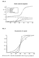
- FIG. 4 illustrates a decomposition of the double sigmoid equation (1).
- the parameters d, e, f and g determine the shape of the two sigmoids.
- the "sharpness" parameters d and f of the double sigmoid equation should be constrained in order to prevent the curve from taking unrealistic shapes. Therefore, in one aspect, any iterations where d ⁇ -1 or d > 1.1 or where f ⁇ -1 or f> 1.1 is considered unsuccessful. In other aspects, different constraints on parameters d and f may be used.
- the Levenberg-Marquardt algorithm is an iterative algorithm, an initial guess for the parameters of the function to fit is typically needed. The better the initial guess, the better the approximation will be and the less likely it is that the algorithm will converge towards a local minimum. Due to the complexity of the double sigmoid function and the various shapes of PCR curves or other growth curves, one initial guess for every parameter may not be sufficient to prevent the algorithm from sometimes converging towards local minima. Therefore, in one aspect, multiple (e.g., three or more) sets of initial parameters are input and the best result is kept. In one aspect, most of the parameters are held constant across the multiple sets of parameters used; only parameters c, d and f may be different for each of the multiple parameter sets. FIG. 6 shows an example of the three curve shapes for the different parameter sets. The choice of these three sets of parameters is indicative of three possible different shapes of curves representing PCR data. It should be understood that more than three sets of parameters may be processed and the best result kept.
- the initial input parameters of the LM method are identified in step 510. These parameters may be input by an operator or calculated. According to one aspect, the parameters are determined or set according to steps 502, 504 and 506 as discussed below.
- the parameter (a) is the height of the baseline; its value is the same for all sets of initial parameters.
- the parameter (a) is assigned the 3rd lowest y-axis value, e.g., fluorescence value, from the data set. This provides for a robust calculation.
- the parameter (a) may be assigned any other fluorescence value as desired such as the lowest y-axis value, second lowest value, etc.
- the parameter (b) is the slope of the baseline and plateau. Its value is the same for all sets of initial parameters. In one aspect, in step 502 a static value of 0.01 is assigned to (b) as ideally there shouldn't be any slope. In other aspects, the parameter (b) may be assigned a different value, for example, a value ranging from 0 to about 0.5.
- the parameter (c) represents the absolute intensity of the curve; for PCR data the parameter (c) typically represents the AFI of the curve. To calculate the AFI, the height of the plateau is important.
- the 3rd highest y-axis value e.g., fluorescence value
- the plateau height is assigned as the plateau height in step 504.
- the parameter (c) may be assigned any other fluorescence value as desired, such as the highest y-axis value, next highest, etc.
- the parameters (d) and (f) define the sharpness of the two sigmoids. As there is no way of giving an approximation based on the curve for these parameters, in one aspect three static representative values are used in step 502. It should be understood that other static or non-static values may be used for parameters (d) and/or (f). These pairs model the most common shapes on PCR curves encountered. Table 2, below, shows the values of (d) and (f) for the different sets of parameters as shown in FIG. 6. Table 2: Values of parameters d and f Parameter set number Value of d Value of f 1 0.1 0.7 2 1.0 0.4 3 0.35 0.25
- the parameters (e) and (g) are determined.
- the parameters (e) and (g) define the inflexion points of the two sigmoids. In one aspect, they both take the same value across all the initial parameter sets. Parameters (e) and (g) may have the same or different values.
- the x-value of the first point above the mean of the intensity, e.g., fluorescence, (which isn't a spike) is used.
- a process for determining the value of (e) and (g) according to this aspect is shown in FIG. 7 and discussed below.
- the mean of the curve e.g., fluorescence intensity
- the first data point above the mean is identified. It is then determined whether:
- Table 3 shows examples of initial parameter values as used in FIG. 6 according to one aspect.
- Table 3 Initial parameters values: Initial parameter set number 1 2 3 Value of a 3 rd lowest fluorescence value 3 rd lowest fluorescence value 3 rd lowest fluorescence value Value of b 0.01 0.01 0.01 Value of c 3 rd highest fluorescence value - a + 2 3 rd highest fluorescence value - a 3 rd highest fluorescence value - a Value of d 0.1 1.0 0.35 Value of e X of the first non-spiky point above the mean of the fluorescence X of the first non-spiky point above the mean of the fluorescence X of the first non-spiky point above the mean of the fluorescence Value of f 0.7 0.4 0.25 Value of g X of the first non-spiky point above the mean of the fluorescence X of the first non-spiky point above the mean of the fluorescence X of the first non-spiky point above the mean of the flu
- a LM process 520 is executed using the input data set, function and parameters.
- the traditional LM method calculates a distance measure defined as the sum of the square of the errors between the curve approximation and the data set.
- the distance between the approximation and the data set is computed by minimizing the sum of absolute errors as this does not give as much weight to the outliers.
- each of the multiple (e.g., three) sets of initial parameters are input and processed and the best result is kept as shown in steps 522 and 524, where the best result is the parameter set that provides the smallest or minimum distance in equation (3).
- most of the parameters are held constant across the multiple sets of parameters; only c, d and f may be different for each set of parameters. It should be understood that any number of initial parameter sets may be used.
- FIG. 8 illustrates a process flow of LM process 520 for a set of parameters according to the present invention.
- the Levenberg-Marquardt method can behave either like a steepest descent process or like a Gauss-Newton process. Its behavior depends on a damping factor ⁇ . The larger ⁇ is, the more the Levenberg-Marquardt algorithm will behave like the steepest descent process. On the other hand, the smaller ⁇ is, the more the Levenberg-Marquardt algorithm will behave like the Gauss-Newton process.
- ⁇ is initiated at 0.001. It should be appreciated that ⁇ may be initiated at any other value, such as from about 0.000001 to about 1.0.
- the Levenberg-Marquardt method is an iterative technique. According to one aspect, as shown in FIG. 8 the following is done during each iteration:
- the LM process of FIG. 8 iterates until one of the following criteria is achieved:
- the curve may be normalized using one or more of the determined parameters.
- the curve may be normalized or adjusted to have zero slope by subtracting out the linear growth portion of the curve.
- dataNew BLS data - a + bx
- dataNew(BLS) is the normalized signal after baseline subtraction, e.g., the data set (data) with the linear growth or baseline slope subtracted off or removed.
- the values of parameters a and b are those values determined by using the LM equation to regress the curve, and x is the cycle number.
- the constant a and the slope b times the x value is subtracted from the data to produce a data curve with a zero slope.
- spike points are removed from the dataset prior to applying the LM regression process to the dataset to determine normalization parameters.
- the value of parameters a and b are those values determined by using the LM equation to regress the curve, and x is the cycle number.
- the constant a and the slope b times the x value is subtracted from the data and the result divided by the value of parameter a to produce a data curve with a zero slope.
- spike points are removed from the dataset prior to applying the LM regression process to the dataset to determine normalization parameters.
- the values are the parameters a and b are those values determined by using the LM equation to regress to curve, and x is the cycle number.
- spike points are removed from the dataset prior to applying the LM regression process to the dataset to determine normalization parameters.
- a root-finding process or method is applied to the normalized curve.
- a root-finding process, algorithm or method is a process whereby the root or roots of a function are determined, typically by iteratively proceeding to improve the solution until a convergence criterion has been satisfied.
- Useful root-finding processes include Newton's method (also known as the Newton-Raphson method), a bisection method, a damped Newton's method, a BFGS, a quasi-Newton method, a secant method, Brent's principal axis method and various variations of these and other root-finding methods.
- the normalized curve is set equal to a function of the AFL value, which function may vary depending on the normalization method used. For example, in order to specify one AFL value for each of the three normalization methods above, additional rules should be implemented to allow for the root-finding process to converge properly, as equations (6) and (7) normalize to "0", and equation (8) normalizes to "1". Accordingly, in one aspect, when equation (8) is used equation (1) is set equal to the AFL value, whereas if equation (6) or (7) is used, equation (1) is set equal to AFL-1. Mathematically, this is shown immediately below for each of the normalization methods of equations (6), (7), and (8).
- the AFL value is typically provided or determined by an assay developer as is well known to one skilled in the art. Further, it should be appreciated that for different assays it may be more advantageous to use different normalization equations. For example, for an HPV assay, it may be more advantageous to use the normalization method according to equation (6) since this type of assay typically has high baselines. For an HCV assay, it may be more advantageous to use a normalization method according to equation (7) or equation (8). One skilled in the art will readily appreciate which normalization method(s) may be more suitable depending on the particular assay.
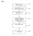
- step 910 the data set is acquired.
- the determination process is implemented in an intelligence module (e.g., processor executing instructions) resident in a PCR data acquiring device such as a thermocycler
- the data set may be provided to the intelligence module in real time as the data is being collected, or it may be stored in a memory unit or buffer and provided to the module after the experiment has been completed.
- the data set may be provided to a separate system such as a desktop computer system via a network connection (e.g., LAN, VPN, intranet, Internet, etc.) or direct connection (e.g., USB or other direct wired or wireless connection) to the acquiring device, or provided on a portable medium such as a CD, DVD, floppy disk or the like.
- a network connection e.g., LAN, VPN, intranet, Internet, etc.
- direct connection e.g., USB or other direct wired or wireless connection
- portable medium such as a CD, DVD, floppy disk or the like.
- step 920 an approximation to the curve is determined.
- a double sigmoid function with parameters determined by a Levenberg Marquardt regression process is used to find an approximation of a curve representing the dataset.
- spike points may be removed from the dataset prior to step 920 as described with reference to FIG. 3.
- the dataset acquired in step 910 can be a dataset with spikes already removed.
- the curve is normalized. In certain aspects, the curve is normalized using one of equations (6), (7), or (8) above.
- the baseline may be set to zero slope using the parameters of the double sigmoid equation as determined in step with 920 to subtract off the baseline slope as per equation (6) above.
- a root-finding method or process is applied to the normalized curve to determine the root, which corresponds to the elbow or Ct value.
- the applied root-finding method may include any of the algorithms discussed above or any other algorithm as would be apparent to one skilled in the art.
- the result is returned, for example to the system that performed the analysis, or to a separate system that requested the analysis.
- Ct value is displayed. Additional data such as the entire data set or the curve approximation may also be displayed.
- Graphical displays may be rendered with a display device, such as a monitor screen or printer, coupled with the system that performed the analysis of FIG. 9, or data may be provided to a separate system for rendering on a display device.
- FIG. 12 Another example of this double sigmoid / LM method is shown in FIG. 12.
- the solid line in FIG. 12 is the double sigmoid/LM curve fit of the data with parameter values shown in Table 2.
- Table 2 Estimate a 1.47037 b 0.00933534 c 10.9464 d 0.79316 e 35.9085 f 0.108165 g 49.193
- a computer implemented method of determining a point at the end of the baseline region of a growth curve typically includes the steps of receiving a dataset representing a growth curve, the dataset including a plurality of data points each having a pair of coordinate values, and calculating an approximation of a curve that fits the dataset by applying a Levenberg-Marquardt (LM) regression process to a double sigmoid function to determine parameters of the function.
- the method further typically includes normalizing the curve using the determined parameters to produce a normalized curve, and processing the normalized curve to determine a coordinate value of a point at the end of the baseline region of the growth curve.
- LM Levenberg-Marquardt
- the dataset represents an amplification growth curve for a kinetic Polymerase Chain Reaction (PCR) process, and the point at the end of the baseline region represents the elbow or cycle threshold (Ct) value for the kinetic PCR curve.
- the dataset represents a growth curve for a kinetic Polymerase Chain Reaction (PCR) process, a bacterial process, an enzymatic process or a binding process.
- the dataset represents a growth curve for a kinetic Polymerase Chain Reaction (PCR) process and the point at the end of the baseline region represents the elbow or cycle threshold (Ct) of the growth curve.
- normalizing includes subtracting off a linear growth portion of the dataset representing a curve.
- processing includes applying a root-finding process to the normalized curve.
- the root-finding process includes a process selected from the group consisting of a Newton's method, a bisection method, a damped Newton's method, a BFGS method, a quasi-Newton method, a secant method and Brent's principal axis method.
- the double sigmoid function is of the form: a + bx + c 1 + exp - d ⁇ x - e ⁇ 1 + exp - f ⁇ x - g , wherein calculating includes iteratively determining one or more of the parameters a, b, c, d, e, f and g of the function.
- at least the parameters a and b are determined and normalizing includes subtracting off the linear growth portion, a+bx, from the curve.
- processing the normalized curve includes applying a root-finding algorithm to the normalized curve and setting the normalized curve equal to the Arbitrary Fluorescence Level (AFL)-1.
- at least the parameters a and b are determined and normalizing includes subtracting off the linear growth portion, a+bx, from the curve and dividing the result by parameter a.
- At least the parameter a is determined and normalizing includes dividing the curve by parameter a.
- processing the normalized curve includes applying a root-finding algorithm to the normalized curve and setting the normalized curve equal to the Arbitrary Fluorescence Level (AFL).
- processing the normalized curve includes applying a root-finding algorithm to the normalized curve and setting the normalized curve equal to the Arbitrary Fluorescence Level (AFL)-1.
- the pair of coordinate values represents an accumulation of amplified polynucleotide and a cycle number.
- the accumulation of amplified polynucleotide is represented by one of a fluorescence intensity value, a luminescence intensity value, a chemiluminescence intensity value, a phosphorescence intensity value, a charge transfer value, a bioluminescence intensity value, or an absorbance value.
- a computer-readable medium including code for controlling a processor to determine a point at the end of the baseline region of a growth curve.
- the code typically includes instructions to receive a dataset representing a growth curve, the dataset including a plurality of data points each having a pair of coordinate values, and calculate an approximation of a curve that fits the dataset by applying a Levenberg-Marquardt (LM) regression process to a double sigmoid function to determine parameters of the function.
- the code also typically includes instructions to normalize the curve using the determined parameters to produce a normalized curve, and process the normalized curve to determine a coordinate value of a point at the end of the baseline region of the growth curve.
- LM Levenberg-Marquardt
- the dataset represents a growth curve for a kinetic Polymerase Chain Reaction (PCR) process, a bacterial process, an enzymatic process or a binding process.
- the curve is an amplification curve for a kinetic Polymerase Chain Reaction (PCR) process
- the point at the end of the baseline region represents the elbow or cycle threshold (Ct) value for the kinetic PCR curve.
- normalizing includes subtracting off a linear growth portion of the curve.
- the code may further include instructions to return or display the coordinate value of the point at the end of the baseline region.
- the pair of coordinate values represents an accumulation of amplified polynucleotide and a cycle number.
- the accumulation of amplified polynucleotide is represented by one of a fluorescence intensity value, a luminescence intensity value, a chemiluminescence intensity value, a phosphorescence intensity value, a charge transfer value, a bioluminescence intensity value, or an absorbance value.
- the instructions to normalize include instructions to subtract off a linear growth portion from the dataset.
- the instructions to process include instructions to apply a root-finding process to the normalized curve.
- the root-finding process includes a process selected from the group consisting of a Newton's method, a bisection method, a damped Newton's method, a BFGS method, a quasi-Newton method, a secant method and Brent's principal axis method.
- the double sigmoid function is of the form:
- the instructions to normalize include instructions to subtract off the linear growth portion, a+bx, from the curve and divide the result by parameter a.
- the instructions to process the normalized curve may include instructions to apply a root-finding algorithm to the normalized curve and to set the normalized curve equal to the Arbitrary Fluorescence Level (AFL)-1.
- the instructions to normalize include instructions to divide the curve by parameter a.
- the instructions to process the normalized curve include instructions to apply a root-finding algorithm to the normalized curve and to set the normalized curve equal to the Arbitrary Fluorescence Level (AFL).
- a kinetic Polymerase Chain Reaction (PCR) system typically includes a kinetic PCR analysis module that generates a PCR dataset representing a kinetic PCR amplification curve, the dataset including a plurality of data points, each having a pair of coordinate values, wherein the dataset includes data points in a region of interest which includes a cycle threshold (Ct) value, and an intelligence module adapted to process the PCR dataset to determine the Ct value.
- a kinetic PCR analysis module that generates a PCR dataset representing a kinetic PCR amplification curve, the dataset including a plurality of data points, each having a pair of coordinate values, wherein the dataset includes data points in a region of interest which includes a cycle threshold (Ct) value
- Ct cycle threshold
- the intelligence module typically processes the PCR dataset by calculating an approximation of a curve that fits the dataset by applying a Levenberg-Marquardt (LM) regression process to a double sigmoid function to determine parameters of the function, by normalizing the curve using the determined parameters to produce a normalized curve, and by processing the normalized curve to determine a coordinate value of a point at the end of the baseline region of the growth curve, wherein the point represents the cycle threshold (Ct) value of the growth curve.
- LM Levenberg-Marquardt
- normalizing includes subtracting off a linear growth portion from the dataset.
- processing includes applying a root-finding process to the normalized curve.
- the root-finding process includes a process selected from the group consisting of a Newton's method, a bisection method, a damped Newton's method, a BFGS method, a quasi-Newton method, a secant method and Brent's principal axis method.
- the pair of coordinate values represent an accumulation of amplified polynucleotide and a cycle number.
- the accumulation of amplified polynucleotide is represented by one of a fluorescence intensity value, a luminescence intensity value, a chemiluminescence intensity value, a phosphorescence intensity value, a charge transfer value, a bioluminescence intensity value, or an absorbance value.
- the kinetic PCR analysis module is resident in a kinetic thermocycler device
- the intelligence module includes a processor communicably coupled to the analysis module.
- the intelligence module includes a processor resident in a computer system coupled to the analysis module by one of a network connection or a direct connection.
- the double sigmoid function is of the form: a + bx + c 1 + exp - d ⁇ x - e ⁇ 1 + exp - f ⁇ x - g , and wherein calculating includes iteratively determining one or more of the parameters a, b, c, d, e, f and g of the function.
- at least the parameters a and b are determined and normalizing includes subtracting off the linear growth portion, a+bx, from the curve.
- processing the normalized curve includes applying a root-finding algorithm to the normalized curve and setting the normalized curve equal to the Arbitrary Fluorescence Level (AFL)-1.
- normalizing includes subtracting off the linear growth portion, a+bx, from the curve and dividing the result by parameter a.
- the normalized curve includes applying a root-finding algorithm to the normalized curve and setting the normalized curve equal to the Arbitrary Fluorescence Level (AFL)-1.
- At least the parameter a is determined and normalizing includes dividing the curve by parameter a.
- processing the normalized curve includes applying a root-finding algorithm to the normalized curve and setting the normalized curve equal to the Arbitrary Fluorescence Level (AFL).
- AFL Arbitrary Fluorescence Level
- the Ct determination processes may be implemented in computer code running on a processor of a computer system.
- the code includes instructions for controlling a processor to implement various aspects and steps of the Ct determination processes.
- the code is typically stored on a hard disk, RAM or portable medium such as a CD, DVD, etc.
- the processes may be implemented in a PCR device such as a thermocycler including a processor executing instructions stored in a memory unit coupled to the processor. Code including such instructions may be downloaded to the PCR device memory unit over a network connection or direct connection to a code source or using a portable medium as is well known.
- elbow determination processes of the present invention can be coded using a variety of programming languages such as C, C++, C#, Fortran, VisualBasic, etc., as well as applications such as Mathematica which provide pre-packaged routines, functions and procedures useful for data visualization and analysis.
- programming languages such as C, C++, C#, Fortran, VisualBasic, etc.
- Mathematica which provide pre-packaged routines, functions and procedures useful for data visualization and analysis.
- Mathematica which provide pre-packaged routines, functions and procedures useful for data visualization and analysis.
- MATLAB ® is a variety of programming languages such as C, C++, C#, Fortran, VisualBasic, etc.
Landscapes
- Engineering & Computer Science (AREA)
- Physics & Mathematics (AREA)
- General Physics & Mathematics (AREA)
- Mathematical Physics (AREA)
- Data Mining & Analysis (AREA)
- Theoretical Computer Science (AREA)
- Mathematical Optimization (AREA)
- Mathematical Analysis (AREA)
- Pure & Applied Mathematics (AREA)
- Computational Mathematics (AREA)
- Algebra (AREA)
- Databases & Information Systems (AREA)
- Software Systems (AREA)
- General Engineering & Computer Science (AREA)
- Measuring Or Testing Involving Enzymes Or Micro-Organisms (AREA)
- Management, Administration, Business Operations System, And Electronic Commerce (AREA)
- Investigating, Analyzing Materials By Fluorescence Or Luminescence (AREA)
Abstract
Description
- The present invention relates generally to systems and methods for processing data representing sigmoid or growth curves, and more particularly to systems and methods for determining characteristic cycle threshold (Ct) or elbow values in PCR amplification curves.
- The Polymerase Chain Reaction (PCR) is an in vitro method for enzymatically synthesizing or amplifying defined nucleic acid sequences. The reaction typically uses two oligonucleotide primers that hybridize to opposite strands and flank a template or target DNA sequence that is to be amplified. Elongation of the primers is catalyzed by a heat-stable DNA polymerase. A repetitive series of cycles involving template denaturation, primer annealing, and extension of the annealed primers by the polymerase results in an exponential accumulation of a specific DNA fragment. Fluorescent probes or markers are typically used in the process to facilitate detection and quantification of the amplification process.
- A typical real-time PCR curve is shown in FIG. 1, where fluorescence intensity values are plotted vs. cycle number for a typical PCR process. In this case, the formation of PCR products is monitored in each cycle of the PCR process. The amplification is usually measured in thermocyclers which include components and devices for measuring fluorescence signals during the amplification reaction. An example of such a thermocycler is the Roche Diagnostics LightCycler (Cat. No. 20110468). The amplification products are, for example, detected by means of fluorescent labeled hybridization probes which only emit fluorescence signals when they are bound to the target nucleic acid or in certain cases also by means of fluorescent dyes that bind to double-stranded DNA.
- For a typical PCR curve, identifying a transition point at the end of the baseline region, which is referred to commonly as the elbow value or cycle threshold (Ct) value, is extremely useful for understanding characteristics of the PCR amplification process. The Ct value may be used as a measure of efficiency of the PCR process. For example, typically a defined signal threshold is determined for all reactions to be analyzed and the number of cycles (Ct) required to reach this threshold value is determined for the target nucleic acid as well as for reference nucleic acids such as a standard or housekeeping gene. The absolute or relative copy numbers of the target molecule can be determined on the basis of the Ct values obtained for the target nucleic acid and the reference nucleic acid (Gibson et al., Genome Research 6:995-1001; Bieche et al., Cancer Research 59:2759-2765, 1999;
WO 97/46707 WO 97/46712 WO 97/46714 cycle number 30. - The elbow value in a PCR curve can be determined using several existing methods. For example, various current methods determine the actual value of the elbow as the value where the fluorescence reaches a predetermined level called the AFL (arbitrary fluorescence value). Other current methods might use the cycle number where the second derivative of fluorescence vs. cycle number reaches a maximum. All of these methods have severe drawbacks. For example, some methods are very sensitive to outlier (noisy) data, and the AFL value approach does not work well for data sets with high baselines. Traditional methods to determine the baseline stop (or end of the baseline) for the growth curve shown in FIG. 1 may not work satisfactorily, especially in a high titer situation. Furthermore, these algorithms typically have many parameters (e.g., 50 or more) that are poorly defined, linearly dependent, and often very difficult, if not impossible, to optimize.
- Therefore it is desirable to provide systems and methods for determining the elbow value in curves, such as sigmoid-type or growth curves, and PCR curves in particular, which overcome the above and other problems.
- The present invention provides novel, efficient systems and methods for determining characteristic transition values such as elbow values in sigmoid or growth-type curves. In one implementation, the systems and methods of the present invention are particularly useful for determining the cycle threshold (Ct) value in PCR amplification curves.
- According to the present invention, a double sigmoid function with parameters determined by a Levenberg-Marquardt (LM) regression process is used to find an approximation to a curve that fits a PCR dataset. Once the parameters have been determined, the curve can be normalized using one or more of the determined parameters. Normalization is advantageous for determining the Ct value if one chooses the arbitrary fluorescence level (AFL) approach to calculating Ct values for amplification curves. After normalization, the normalized curve is processed by applying a root-finding algorithm to determine the root of the function representing the normalized curve, which root corresponds to the Ct value. The Ct value is then returned and may be displayed or otherwise used for further processing.
- In a first aspect of the invention a computer implemented method of determining a point at the end of the baseline region of a growth curve is provided, comprising the steps of:
- receiving a dataset representing a growth curve, said dataset including a plurality of data points each having a pair of coordinate values;
- calculating an approximation of a curve that fits the dataset by applying a Levenberg-Marquardt (LM) regression process to a double sigmoid function to determine parameters of the function;
- normalizing the curve using the determined parameters to produce a normalized curve; and
- processing the normalized curve to determine a coordinate value of a point at the end of the baseline region of the growth curve.
- In a second aspect of the invention a computer-readable medium including code for controlling a processor to determine a point at the end of the baseline region of a growth curve is provided, wherein the code includs instructions to:
- receive a dataset representing a growth curve, said dataset including a plurality of data points each having a pair of coordinate values;
- calculate an approximation of a curve that fits the dataset by applying a Levenberg-Marquardt (LM) regression process to a double sigmoid function to determine parameters of the function;
- normalize the curve using the determined parameters to produce a normalized curve; and
- process the normalized curve to determine a coordinate value of a point at the end of the baseline region of the growth curve.
- In yet another aspect of the invention a kinetic Polymerase Chain Reaction (PCR) system is provided, comprising:
- a kinetic PCR analysis module that generates a PCR dataset representing a kinetic PCR amplification curve, said dataset including a plurality of data points, each having a pair of coordinate values, wherein said dataset includes data points in a region of interest which includes a cycle threshold (Ct) value; and
- an intelligence module adapted to process the PCR dataset to determine the Ct value, by:
- calculating an approximation of a curve that fits the dataset by applying a Levenberg-Marquardt (LM) regression process to a double sigmoid function to determine parameters of the function;
- normalizing the curve using the determined parameters to produce a normalized curve; and
- processing the normalized curve to determine a coordinate value of a point at the end of the baseline region of the growth curve, wherein said point represents the cycle threshold (Ct) value of the growth curve.
-
- FIG. 1 illustrates an example of a typical PCR growth curve, plotted as fluorescence intensity vs. cycle number.
- FIG. 2 shows a process flow for determining the end of a baseline region of a growth curve, or Ct value of a PCR curve.
- FIG. 3 illustrates a detailed process flow for a spike identification and replacement process according to one embodiment of the present invention.
- FIG. 4 illustrates a decomposition of the double sigmoid equation including parameters a-g.
- FIG. 5 shows the influence of parameter (d) on the curve and the position of (e), the x value of the inflexion point.
- FIG. 6 shows an example of the three curve shapes for the different parameter sets.
- FIG. 7 illustrates a process for determining the value of double sigmoid equation parameters (e) and (g) according to one aspect.
- FIG. 8 illustrates a process flow of a Levenberg-Marquardt regression process for an initial set of parameters.
- FIG. 9 illustrates a more detailed process flow for determining the elbow value for a PCR process according to one embodiment.
- FIG. 10 shows a plot of a PCR dataset.
- FIG. 11 shows the data set of FIG. 10 after normalization using the baseline subtraction with division method of equation (7).
- FIG. 12 shows a plot of another PCR dataset.
- FIG. 13 shows the data set of FIG. 12 after normalization using the baseline subtraction with division method of equation (7).
- FIG. 14 shows a general block diagram depicting the relation between the software and hardware resources.
- The present invention provides systems and methods for determining a transition value in a sigmoid or growth curve, such as the end of the baseline region or the elbow value or Ct value of a kinetic PCR amplification curve. In certain aspects, a double sigmoid function with parameters determined by a Levenberg-Marquardt (LM) regression process is used to find an approximation to the curve. Once the parameters have been determined, the curve can be normalized using one or more of the determined parameters. Normalization is advantageous for determining the Ct value if one chooses the arbitrary fluorescence level (AFL) approach to calculating Ct values for amplification curves. After normalization, the normalized curve is processed by applying a root-finding algorithm to determine the root of the function representing the normalized curve, which root corresponds to the Ct value. The Ct value is then returned and may be displayed or otherwise used for further processing. One example of an
amplification curve 10 in the context of a PCR process is shown in FIG. 1. As shown, thecurve 10 includes alag phase region 15, and anexponential phase region 25.Lag phase region 15 is commonly referred to as the baseline or baseline region. Such acurve 10 includes a transitionary region ofinterest 20 linking the lag phase and the exponential phase regions.Region 20 is commonly referred to as the elbow or elbow region. The elbow region typically defines an end to the baseline and a transition in the growth or amplification rate of the underlying process. Identifying a specific transition point inregion 20 can be useful for analyzing the behavior of the underlying process. In a typical PCR curve, identifying a transition point referred to as the elbow value or cycle threshold (Ct) value is extremely useful for understanding efficiency characteristics of the PCR process. - Other processes that may provide similar sigmoid or growth curves include bacterial processes, enzymatic processes and binding processes. In bacterial growth curves, for example, the transition point of interest has been referred to as the time in lag phase, θ. Other specific processes that produce data curves that may be analyzed according to the present invention include strand displacement amplification (SDA) processes, nucleic acid sequence-based amplification (NASBA) processes and transcription mediated amplification (TMA) processes. Examples of SDA and NASBA processes and data curves can be found in Wang, Sha-Sha, et al., "Homogeneous Real-Time Detection of Single-Nucleotide Polymorphisms by Strand Displacement Amp lification on the BD ProbeTec ET System", Clin Chem 2003 49(10):1599, and Weusten, Jos J.A.M., et al., "Principles of Quantitation of Viral Loads Using Nucleic Acid Sequence-Based Amplification in Combination With Homogeneous Detection Using Molecular Beacons", Nucleic Acids Research, 2002 30(6):26, respectively. Thus, although the remainder of this document will discuss embodiments and aspects of the invention in terms of its applicability to PCR curves, it should be appreciated that the present invention may be applied to data curves related to other processes.
- As shown in FIG. 1, data for a typical PCR growth curve can be represented in a two-dimensional coordinate system, for example, with PCR cycle number defining the x-axis and an indicator of accumulated polynucleotide growth defining the y-axis. Typically, as shown in FIG. 1, the indicator of accumulated growth is a fluorescence intensity value as the use of fluorescent markers is perhaps the most widely used labeling scheme. However, it should be understood that other indicators may be used depending on the particular labeling and/or detection scheme used. Examples of other useful indicators of accumulated signal growth include luminescence intensity, chemiluminescence intensity, bioluminescence intensity, phosphorescence intensity, charge transfer, voltage, current, power, energy, temperature, viscosity, light scatter, radioactive intensity, reflectivity, transmittance and absorbance. The definition of cycle can also include time, process cycles, unit operation cycles and reproductive cycles.
- According to the present invention, one embodiment of a
process 100 for determining a transitionary value in a single sigmoid curve, such as the elbow value or Ct value of a kinetic PCR amplification curve, can be described briefly with reference to FIG. 2. Instep 110, an experimental data set representing the curve is received or otherwise acquired. An example of a plotted PCR data set is shown in FIG. 1, where the y-axis and x-axis represent fluorescence intensity and cycle number, respectively, for a PCR curve. In certain aspects, the data set should include data that is continuous and equally spaced along an axis. - In an exemplary embodiment of the present invention, the method may be implemented by using conventional personal computer systems including, but not limited to, an input device to input a data set, such as a keyboard, mouse, and the like; a display device to represent a specific point of interest in a region of a curve, such as a monitor; a processing device necessary to carry out each step in the method, such as a CPU; a network interface such as a modem a data storage device to store the data set, a computer code running on the processor and the like. Furthermore, the method may also be implemented in a PCR device.
- A system according to the invention is displayed in FIG. 14. This figure shows a general block diagram explaining the relation between the software and hardware resources. The system comprises a kinetic PCR analysis module which may be located in a thermocycler device and an intelligence module which is part of the computer system. The data sets (PCR data sets) are transferred from the analysis module to the intelligence module or vice versa via a network connection or a direct connection. The data sets are processed according to the method as displayed in Fig. 2 by computer code running on the processor and being stored on the storage device of the intelligence module and after processing transferred back to the storage device of the analysis module, where the modified data may be displayed on a displaying device. In a particular embodiment the intelligence module may also be implemented in the PCR data acquiring device.
- In the case where
process 100 is implemented in an intelligence module (e.g., processor executing instructions) resident in a PCR data acquiring device such as a thermocycler, the data set may be provided to the intelligence module in real time as the data is being collected, or it may be stored in a memory unit or buffer and provided to the intelligence module after the experiment has been completed. Similarly, the data set may be provided to a separate system such as a desktop computer system or other computer system, via a network connection (e.g., LAN, VPN, intranet, Internet, etc.) or direct connection (e.g., USB or other direct wired or wireless connection) to the acquiring device, or provided on a portable medium such as a CD, DVD, floppy disk or the like. In certain aspects, the data set includes data points having a pair of coordinate values (or a 2-dimensional vector). For PCR data, the pair of coordinate values typically represents the cycle number and the fluorescence intensity value. After the data set has been received or acquired instep 110, the data set may be analyzed to determine the end of the baseline region. - In
step 120, an approximation of the curve is calculated. During this step, in one embodiment, a double sigmoid function with parameters determined by a Levenberg-Marquardt (LM) regression process or other regression process is used to find an approximation of a curve representing the data set. The approximation is said to be "robust" as outlier or spike points have a minimal effect on the quality of the curve fit. FIG 2 illustrates a plot of the received data set and a robust approximation of the data set determined by using a Levenberg-Marquardt regression process to determine the parameters of a double sigmoid function according to the present invention. - In certain aspects, outlier or spike points in the dataset are removed or replaced prior to processing the data set to determine the end of the baseline region. Spike a removal may occur before or after the dataset is acquired in
step 110. FIG. 3 illustrates the process flow for identifying and replacing spike points in datasets representing PCR or other growth curves. - In
step 130, the parameters determined instep 120 are used to normalize the curve, as will be described in more detail below. Normalization in this manner allows for determining the Ct value without having to determine or specify the end of the baseline region of the curve or a baseline stop position. Instep 140, the normalized curve is then processed to determine the Ct value as will be discussed in more detail below. -
Steps 502 through 524 of FIG. 3 also illustrate a process flow for approximating the curve of a dataset and determining the parameters of a fit function (step 120). These parameters can be used in normalizing the curve, e.g., modifying or removing the baseline slope of the data set representing a sigmoid or growth type curve such as a PCR curve according to one embodiment of the present invention (step 130). Where the dataset has been processed to produce a modified dataset with removed or replaced spike points, the modified spikeless dataset may be processed according tosteps 502 through 524 to identify the parameters of the fit function. - In one embodiment as shown, a Levenberg-Marquardt (LM) method is used to calculate a robust curve approximation of a data set. The LM method is a non-linear regression process; it is an iterative technique that minimizes the distance between a non-linear function and a data set. The process behaves like a combination of a steepest descent process and a Gauss-Newton process: when the current approximation doesn't fit well it behaves like the steepest descent process (slower but more reliable convergence), but as the current approximation becomes more accurate it will then behave like the Gauss-Newton process (faster but less reliable convergence). The LM regression method is widely used to solve non-linear regression problems.
- In general, the LM regression method includes an algorithm that requires various inputs and provides output. In one aspect, the inputs include a data set to be processed, a function that is used to fit the data, and an initial guess for the parameters or variables of the function. The output includes a set of parameters for the function that minimizes the distance between the function and the data set.
- According to one embodiment, the fit function is a double sigmoid of the form:

- The choice of this equation as the fit function is based on its flexibility and its ability to fit the different curve shapes that a typical PCR curve or other growth curve may take. One skilled in the art will appreciate that variations of the above fit function or other fit functions may be used as desired.
- The double sigmoid equation (1) has 7 parameters: a, b, c, d, e, f and g. The equation can be decomposed into a sum of a constant, a slope and a double sigmoid. The double sigmoid itself is the multiplication of two sigmoids. FIG. 4 illustrates a decomposition of the double sigmoid equation (1). The parameters d, e, f and g determine the shape of the two sigmoids. To show their influence on the final curve, consider the single sigmoid:

where the parameter d determines the "sharpness" of the curve and the parameter e determines the x-value of the inflexion point. FIG. 5 shows the influence of the parameter d on the curve and of the parameter e on the position of the x value of the inflexion point. Table 1, below, describes the influence of the parameters on the double sigmoid curve.Table 1: Double sigmoid parameters description Parameter Influence on the curve a Value of y at x = 0 b baseline and plateau slope c AFI of the curve d "sharpness" of the first sigmoid (See Figure. 7) e position of the inflexion point of the first sigmoid (See Figure. 7) f "sharpness" of the second sigmoid g position of the inflexion point of the second sigmoid - In one aspect, the "sharpness" parameters d and f of the double sigmoid equation should be constrained in order to prevent the curve from taking unrealistic shapes. Therefore, in one aspect, any iterations where d<-1 or d > 1.1 or where f<-1 or f> 1.1 is considered unsuccessful. In other aspects, different constraints on parameters d and f may be used.
- Because the Levenberg-Marquardt algorithm is an iterative algorithm, an initial guess for the parameters of the function to fit is typically needed. The better the initial guess, the better the approximation will be and the less likely it is that the algorithm will converge towards a local minimum. Due to the complexity of the double sigmoid function and the various shapes of PCR curves or other growth curves, one initial guess for every parameter may not be sufficient to prevent the algorithm from sometimes converging towards local minima. Therefore, in one aspect, multiple (e.g., three or more) sets of initial parameters are input and the best result is kept. In one aspect, most of the parameters are held constant across the multiple sets of parameters used; only parameters c, d and f may be different for each of the multiple parameter sets. FIG. 6 shows an example of the three curve shapes for the different parameter sets. The choice of these three sets of parameters is indicative of three possible different shapes of curves representing PCR data. It should be understood that more than three sets of parameters may be processed and the best result kept.
- As shown in FIG. 3, the initial input parameters of the LM method are identified in
step 510. These parameters may be input by an operator or calculated. According to one aspect, the parameters are determined or set according tosteps - The parameter (a) is the height of the baseline; its value is the same for all sets of initial parameters. In one aspect, in
step 504 the parameter (a) is assigned the 3rd lowest y-axis value, e.g., fluorescence value, from the data set. This provides for a robust calculation. In other aspects, of course, the parameter (a) may be assigned any other fluorescence value as desired such as the lowest y-axis value, second lowest value, etc. - The parameter (b) is the slope of the baseline and plateau. Its value is the same for all sets of initial parameters. In one aspect, in step 502 a static value of 0.01 is assigned to (b) as ideally there shouldn't be any slope. In other aspects, the parameter (b) may be assigned a different value, for example, a value ranging from 0 to about 0.5.
- The parameter (c) represents the absolute intensity of the curve; for PCR data the parameter (c) typically represents the AFI of the curve. To calculate the AFI, the height of the plateau is important.
- To calculate this in a robust way, in one aspect, the 3rd highest y-axis value, e.g., fluorescence value, is assigned as the plateau height in
step 504. Then, the AFI = height of plateau - height of baseline = 3rd highest fluorescence value - (a). In other aspects, the parameter (c) may be assigned any other fluorescence value as desired, such as the highest y-axis value, next highest, etc. - As shown in FIG. 6, for the last two sets of parameters, c = AFI. For the first set of parameters, c =
AFI+ 2. This change is due to the shape of the curve modeled by the first set of parameters, which doesn't have a plateau. - The parameters (d) and (f) define the sharpness of the two sigmoids. As there is no way of giving an approximation based on the curve for these parameters, in one aspect three static representative values are used in
step 502. It should be understood that other static or non-static values may be used for parameters (d) and/or (f). These pairs model the most common shapes on PCR curves encountered. Table 2, below, shows the values of (d) and (f) for the different sets of parameters as shown in FIG. 6.Table 2: Values of parameters d and f Parameter set number Value of d Value of f 1 0.1 0.7 2 1.0 0.4 3 0.35 0.25 - In
step 506, the parameters (e) and (g) are determined. The parameters (e) and (g) define the inflexion points of the two sigmoids. In one aspect, they both take the same value across all the initial parameter sets. Parameters (e) and (g) may have the same or different values. To find an approximation, in one aspect, the x-value of the first point above the mean of the intensity, e.g., fluorescence, (which isn't a spike) is used. A process for determining the value of (e) and (g) according to this aspect is shown in FIG. 7 and discussed below. - With reference to FIG. 7, initially, the mean of the curve (e.g., fluorescence intensity) is determined. Next, the first data point above the mean is identified. It is then determined whether:
- a. that point does not lie near the beginning, e.g., within the first 5 cycles, of the curve;
- b. that point does not lie near the end, e.g., within the 5 last cycles, of the curve; and
- c. the derivatives around the point (e.g., in a radius of 2 points around it) do not show any change of sign. If they do, the point is likely to be a spike and should therefore be rejected.
- Table 3, below, shows examples of initial parameter values as used in FIG. 6 according to one aspect.
Table 3: Initial parameters values: Initial parameter set number 1 2 3 Value of a 3rd lowest fluorescence value 3rd lowest fluorescence value 3rd lowest fluorescence value Value of b 0.01 0.01 0.01 Value of c 3rd highest fluorescence value - a + 2 3rd highest fluorescence value - a 3rd highest fluorescence value - a Value of d 0.1 1.0 0.35 Value of e X of the first non-spiky point above the mean of the fluorescence X of the first non-spiky point above the mean of the fluorescence X of the first non-spiky point above the mean of the fluorescence Value of f 0.7 0.4 0.25 Value of g X of the first non-spiky point above the mean of the fluorescence X of the first non-spiky point above the mean of the fluorescence X of the first non-spiky point above the mean of the fluorescence - Returning to FIG. 3, once all the parameters are set in
step 510, a LM process 520 is executed using the input data set, function and parameters. Traditionally, the Levenberg-Marquardt method is used to solve non-linear least-square problems. The traditional LM method calculates a distance measure defined as the sum of the square of the errors between the curve approximation and the data set. However, when minimizing the sum of the squares, it gives outliers an important weight as their distance is larger than the distance of non-spiky data points, often resulting in inappropriate curves or less desirable curves. Therefore, according to one aspect of the present invention, the distance between the approximation and the data set is computed by minimizing the sum of absolute errors as this does not give as much weight to the outliers. In this aspect, the distance between the approximation and data is given by:
- As above, in one aspect, each of the multiple (e.g., three) sets of initial parameters are input and processed and the best result is kept as shown in steps 522 and 524, where the best result is the parameter set that provides the smallest or minimum distance in equation (3). In one aspect, most of the parameters are held constant across the multiple sets of parameters; only c, d and f may be different for each set of parameters. It should be understood that any number of initial parameter sets may be used.
- FIG. 8 illustrates a process flow of LM process 520 for a set of parameters according to the present invention. As explained above, the Levenberg-Marquardt method can behave either like a steepest descent process or like a Gauss-Newton process. Its behavior depends on a damping factor λ. The larger λ is, the more the Levenberg-Marquardt algorithm will behave like the steepest descent process. On the other hand, the smaller λ is, the more the Levenberg-Marquardt algorithm will behave like the Gauss-Newton process. In one aspect, λ is initiated at 0.001. It should be appreciated that λ may be initiated at any other value, such as from about 0.000001 to about 1.0.
- As stated before, the Levenberg-Marquardt method is an iterative technique. According to one aspect, as shown in FIG. 8 the following is done during each iteration:
- 1. The Hessian Matrix (H) of the precedent approximation is calculated.
- 2. The transposed Jacobian Matrix (JT) of the precedent approximation is calculated.
- 3. The distance vector (d) of the precedent approximation is calculated.
- 4. The Hessian Matrix diagonal is augmented by the current damping factor λ:

- 5. Solve the augmented equation:

- 6. The solution x of the augmented equation is added to the parameters of the function.
- 7. Calculate the distance between the new approximation and the curve.
- 8. If the distance with this new set of parameters is smaller than the distance with the previous set of parameters:
- The iteration is considered successful.
- Keep or store the new set of parameters.
- Decrease the damping factor λ, e.g., by a
factor 10.
- The iteration is considered unsuccessful.
- Throw away the new set of parameters.
- Increase the damping factor λ, e.g., by a factor of 10.
- In one aspect, the LM process of FIG. 8 iterates until one of the following criteria is achieved:
- 1. It has run for a specified number, N, of iterations. This first criterion prevents the algorithm from iterating indefinitely. For example, in one aspect as shown in FIG. 10, the default iteration value N is 100. 100 iterations should be plenty for the algorithm to converge if it can converge. In general, N can range from fewer than 10 to 100 or more.
- 2. The difference of the distances between two successful iterations is smaller than a threshold value. e.g., 0.0001. When the difference becomes very small, the desired precision has been achieved and continuing to iterate is pointless as the solution won't become significantly better.
- 3. The damping factor λ exceeds a specified value, e.g., is larger than 1020. When λ becomes very large, the algorithm won't converge any better than the current solution, therefore it is pointless to continue iterating. In general, the specified value can be significantly smaller or larger than 1020.
- After the parameters have been determined, the curve may be normalized using one or more of the determined parameters. For example, in one aspect, the curve may be normalized or adjusted to have zero slope by subtracting out the linear growth portion of the curve. Mathematically, this is shown as:

where dataNew(BLS) is the normalized signal after baseline subtraction, e.g., the data set (data) with the linear growth or baseline slope subtracted off or removed. The values of parameters a and b are those values determined by using the LM equation to regress the curve, and x is the cycle number. Thus, for every data value along the x-axis, the constant a and the slope b times the x value is subtracted from the data to produce a data curve with a zero slope. In certain aspects, spike points are removed from the dataset prior to applying the LM regression process to the dataset to determine normalization parameters. - In another aspect, the curve may be normalized or adjusted to have zero slope according to the following equation:

where dataNew(BLSD) is the normalized signal after baseline subtraction with division, e.g., the data set (data) with the linear growth or baseline slope subtracted off or removed and the result divided by a. The value of parameters a and b are those values determined by using the LM equation to regress the curve, and x is the cycle number. Thus, for every data value along the x-axis, the constant a and the slope b times the x value is subtracted from the data and the result divided by the value of parameter a to produce a data curve with a zero slope. In certain aspects, spike points are removed from the dataset prior to applying the LM regression process to the dataset to determine normalization parameters. - In yet another aspect, the curve may be normalized or adjusted according to following equation:

where dataNew(BLD) is the normalized signal after baseline division, e.g., the data set (data) divided by parameter a. The values are the parameters a and b are those values determined by using the LM equation to regress to curve, and x is the cycle number. In certain aspects, spike points are removed from the dataset prior to applying the LM regression process to the dataset to determine normalization parameters. - One skilled in the art will appreciate that other normalization equations may be used to normalized and/or modify the baseline using the parameters as determined by the Levenberg-Marquardt or other regression process.
- After the curve has been normalized using one of equations (6), (7) or (8), or other normalization equation, the Ct value can be determined. In one aspect, a root-finding process or method is applied to the normalized curve. A root-finding process, algorithm or method is a process whereby the root or roots of a function are determined, typically by iteratively proceeding to improve the solution until a convergence criterion has been satisfied. Useful root-finding processes include Newton's method (also known as the Newton-Raphson method), a bisection method, a damped Newton's method, a BFGS, a quasi-Newton method, a secant method, Brent's principal axis method and various variations of these and other root-finding methods. Examples of these and other root-finding methods can be found in
Chapter 9 of "Numerical Recipes In C: The Art of Scientific Computing" by Cambridge University Press (ISBN 0-521-43108-5 - In certain aspects, the normalized curve is set equal to a function of the AFL value, which function may vary depending on the normalization method used. For example, in order to specify one AFL value for each of the three normalization methods above, additional rules should be implemented to allow for the root-finding process to converge properly, as equations (6) and (7) normalize to "0", and equation (8) normalizes to "1". Accordingly, in one aspect, when equation (8) is used equation (1) is set equal to the AFL value, whereas if equation (6) or (7) is used, equation (1) is set equal to AFL-1. Mathematically, this is shown immediately below for each of the normalization methods of equations (6), (7), and (8). In one aspect, when the baseline subtraction method of equation (6) is used, a root-finding process or method is applied to the following equation:

- In one aspect, when the baseline subtraction with division method of equation (7) is used, a root-finding process or method is applied to the following equation:

- In one aspect, when the baseline division method of equation (8) is used, a root-finding process or method is applied to the following equation:

- It should be appreciated that the AFL value is typically provided or determined by an assay developer as is well known to one skilled in the art. Further, it should be appreciated that for different assays it may be more advantageous to use different normalization equations. For example, for an HPV assay, it may be more advantageous to use the normalization method according to equation (6) since this type of assay typically has high baselines. For an HCV assay, it may be more advantageous to use a normalization method according to equation (7) or equation (8). One skilled in the art will readily appreciate which normalization method(s) may be more suitable depending on the particular assay.
- A more detailed process flow for determining the elbow value or Ct value in a kinetic PCR curve according to one embodiment is shown in FIG. 9. In
step 910, the data set is acquired. In the case where the determination process is implemented in an intelligence module (e.g., processor executing instructions) resident in a PCR data acquiring device such as a thermocycler, the data set may be provided to the intelligence module in real time as the data is being collected, or it may be stored in a memory unit or buffer and provided to the module after the experiment has been completed. Similarly, the data set may be provided to a separate system such as a desktop computer system via a network connection (e.g., LAN, VPN, intranet, Internet, etc.) or direct connection (e.g., USB or other direct wired or wireless connection) to the acquiring device, or provided on a portable medium such as a CD, DVD, floppy disk or the like. - After a data set has been received or acquired, in
step 920 an approximation to the curve is determined. During this step, in one embodiment, a double sigmoid function with parameters determined by a Levenberg Marquardt regression process is used to find an approximation of a curve representing the dataset. Additionally, spike points may be removed from the dataset prior to step 920 as described with reference to FIG. 3. For example, the dataset acquired instep 910 can be a dataset with spikes already removed. Instep 930, the curve is normalized. In certain aspects, the curve is normalized using one of equations (6), (7), or (8) above. For example, the baseline may be set to zero slope using the parameters of the double sigmoid equation as determined in step with 920 to subtract off the baseline slope as per equation (6) above. Instep 940, a root-finding method or process is applied to the normalized curve to determine the root, which corresponds to the elbow or Ct value. The applied root-finding method may include any of the algorithms discussed above or any other algorithm as would be apparent to one skilled in the art. Instep 950, the result is returned, for example to the system that performed the analysis, or to a separate system that requested the analysis. Instep 960, Ct value is displayed. Additional data such as the entire data set or the curve approximation may also be displayed. Graphical displays may be rendered with a display device, such as a monitor screen or printer, coupled with the system that performed the analysis of FIG. 9, or data may be provided to a separate system for rendering on a display device. - Applying the double sigmoid/LM method to the data shown in FIG. 10 gives values of the seven parameters in equation (1) as shown in Table 1 below:
Table 1 a 8.74168 b 0.0391099 c 51.7682 d 0.250381 e 8.09951 f 0.548204 g 15.7799 - These data were then normalized according to equation (7) (Baseline subtraction with division) to yield the graph shown in FIG. 11. The solid line shown in FIG. 11 is the double sigmoid/LM application of equation (1) to the data set that has been normalized according to equation (7). The AFL value for this case is 1.5, so using equation (10) with AFL-1 equal to 0.5 and using a BFGS quasi-Newton method to find the root, gives a Ct value of 12.07.
- Another example of this double sigmoid / LM method is shown in FIG. 12. The solid line in FIG. 12 is the double sigmoid/LM curve fit of the data with parameter values shown in Table 2.
Table 2 Estimate a 1.47037 b 0.00933534 c 10.9464 d 0.79316 e 35.9085 f 0.108165 g 49.193 - After applying the normalization equation (7) to this data set, the result is shown in FIG. 13, along with the double sigmoid /LM curve fit. The parameter values for this case are shown in Table 2. The AFL value for this case is 1.5, so using equation (10) with AFL-1 equal to 0.5 and using a BFGS quasi-Newton method to find the root, gives a Ct value of 35.24.
- According to one aspect of the present invention, a computer implemented method of determining a point at the end of the baseline region of a growth curve is provided. The method typically includes the steps of receiving a dataset representing a growth curve, the dataset including a plurality of data points each having a pair of coordinate values, and calculating an approximation of a curve that fits the dataset by applying a Levenberg-Marquardt (LM) regression process to a double sigmoid function to determine parameters of the function. The method further typically includes normalizing the curve using the determined parameters to produce a normalized curve, and processing the normalized curve to determine a coordinate value of a point at the end of the baseline region of the growth curve. In one aspect, the dataset represents an amplification growth curve for a kinetic Polymerase Chain Reaction (PCR) process, and the point at the end of the baseline region represents the elbow or cycle threshold (Ct) value for the kinetic PCR curve. In other aspects of the invention the dataset represents a growth curve for a kinetic Polymerase Chain Reaction (PCR) process, a bacterial process, an enzymatic process or a binding process. In a particular embodiment the dataset represents a growth curve for a kinetic Polymerase Chain Reaction (PCR) process and the point at the end of the baseline region represents the elbow or cycle threshold (Ct) of the growth curve.
- In certain aspects of the invention, normalizing includes subtracting off a linear growth portion of the dataset representing a curve. In a certain embodiment, processing includes applying a root-finding process to the normalized curve. In another embodiment the root-finding process includes a process selected from the group consisting of a Newton's method, a bisection method, a damped Newton's method, a BFGS method, a quasi-Newton method, a secant method and Brent's principal axis method.
- In certain aspects, the double sigmoid function is of the form:

- In another embodiment at least the parameter a is determined and normalizing includes dividing the curve by parameter a. In a certain embodiment processing the normalized curve includes applying a root-finding algorithm to the normalized curve and setting the normalized curve equal to the Arbitrary Fluorescence Level (AFL). In another certain embodiment processing the normalized curve includes applying a root-finding algorithm to the normalized curve and setting the normalized curve equal to the Arbitrary Fluorescence Level (AFL)-1. In a yet another certain embodiment the pair of coordinate values represents an accumulation of amplified polynucleotide and a cycle number. In a particular embodiment the accumulation of amplified polynucleotide is represented by one of a fluorescence intensity value, a luminescence intensity value, a chemiluminescence intensity value, a phosphorescence intensity value, a charge transfer value, a bioluminescence intensity value, or an absorbance value.
- According to another aspect of the present invention, a computer-readable medium including code for controlling a processor to determine a point at the end of the baseline region of a growth curve is provided. The code typically includes instructions to receive a dataset representing a growth curve, the dataset including a plurality of data points each having a pair of coordinate values, and calculate an approximation of a curve that fits the dataset by applying a Levenberg-Marquardt (LM) regression process to a double sigmoid function to determine parameters of the function. The code also typically includes instructions to normalize the curve using the determined parameters to produce a normalized curve, and process the normalized curve to determine a coordinate value of a point at the end of the baseline region of the growth curve. In one aspect, the dataset represents a growth curve for a kinetic Polymerase Chain Reaction (PCR) process, a bacterial process, an enzymatic process or a binding process. In a particular aspect the curve is an amplification curve for a kinetic Polymerase Chain Reaction (PCR) process, and the point at the end of the baseline region represents the elbow or cycle threshold (Ct) value for the kinetic PCR curve. In certain aspects, normalizing includes subtracting off a linear growth portion of the curve. In certain aspects the code may further include instructions to return or display the coordinate value of the point at the end of the baseline region.
- In certain embodiments the pair of coordinate values represents an accumulation of amplified polynucleotide and a cycle number. In particular embodiments the accumulation of amplified polynucleotide is represented by one of a fluorescence intensity value, a luminescence intensity value, a chemiluminescence intensity value, a phosphorescence intensity value, a charge transfer value, a bioluminescence intensity value, or an absorbance value.
- In a certain embodiment the instructions to normalize include instructions to subtract off a linear growth portion from the dataset. In another certain embodiment the instructions to process include instructions to apply a root-finding process to the normalized curve. In a particular embodiment the root-finding process includes a process selected from the group consisting of a Newton's method, a bisection method, a damped Newton's method, a BFGS method, a quasi-Newton method, a secant method and Brent's principal axis method.
- In certain aspects, the double sigmoid function is of the form:
-

- In another particular embodiment, wherein at least the parameters a and b are determined, the instructions to normalize include instructions to subtract off the linear growth portion, a+bx, from the curve and divide the result by parameter a. Particularly the instructions to process the normalized curve may include instructions to apply a root-finding algorithm to the normalized curve and to set the normalized curve equal to the Arbitrary Fluorescence Level (AFL)-1.
- In other certain aspects, at least the parameter a is determined the instructions to normalize include instructions to divide the curve by parameter a. In a particular embodiment the instructions to process the normalized curve include instructions to apply a root-finding algorithm to the normalized curve and to set the normalized curve equal to the Arbitrary Fluorescence Level (AFL).
- According to yet another aspect of the present invention, a kinetic Polymerase Chain Reaction (PCR) system is provided. The system typically includes a kinetic PCR analysis module that generates a PCR dataset representing a kinetic PCR amplification curve, the dataset including a plurality of data points, each having a pair of coordinate values, wherein the dataset includes data points in a region of interest which includes a cycle threshold (Ct) value, and an intelligence module adapted to process the PCR dataset to determine the Ct value. The intelligence module typically processes the PCR dataset by calculating an approximation of a curve that fits the dataset by applying a Levenberg-Marquardt (LM) regression process to a double sigmoid function to determine parameters of the function, by normalizing the curve using the determined parameters to produce a normalized curve, and by processing the normalized curve to determine a coordinate value of a point at the end of the baseline region of the growth curve, wherein the point represents the cycle threshold (Ct) value of the growth curve.
- In a certain embodiment of the system according to the invention normalizing includes subtracting off a linear growth portion from the dataset. In another certain embodiment processing includes applying a root-finding process to the normalized curve. In a particular embodiment the root-finding process includes a process selected from the group consisting of a Newton's method, a bisection method, a damped Newton's method, a BFGS method, a quasi-Newton method, a secant method and Brent's principal axis method.
- In another aspect the pair of coordinate values represent an accumulation of amplified polynucleotide and a cycle number. In certain embodiments the accumulation of amplified polynucleotide is represented by one of a fluorescence intensity value, a luminescence intensity value, a chemiluminescence intensity value, a phosphorescence intensity value, a charge transfer value, a bioluminescence intensity value, or an absorbance value.
- In certain embodiments the kinetic PCR analysis module is resident in a kinetic thermocycler device, and the intelligence module includes a processor communicably coupled to the analysis module. In particular embodiments the intelligence module includes a processor resident in a computer system coupled to the analysis module by one of a network connection or a direct connection.
- In a certain aspect, the double sigmoid function is of the form:

- In another embodiment, wherein at least the parameters a and b are determined, normalizing includes subtracting off the linear growth portion, a+bx, from the curve and dividing the result by parameter a. In a particular embodiment the normalized curve includes applying a root-finding algorithm to the normalized curve and setting the normalized curve equal to the Arbitrary Fluorescence Level (AFL)-1.
- In another certain embodiment at least the parameter a is determined and normalizing includes dividing the curve by parameter a. In a particular embodiment processing the normalized curve includes applying a root-finding algorithm to the normalized curve and setting the normalized curve equal to the Arbitrary Fluorescence Level (AFL).
- Reference to the remaining portions of the specification, including the drawings and claims, will realize other features and advantages of the present invention. Further features and advantages of the present invention, as well as the structure and operation of various embodiments of the present invention, are described in detail below with respect to the accompanying drawings. In the drawings, like reference numbers indicate identical or functionally similar elements.
- It should be appreciated that the Ct determination processes, including the curve approximation and root-finding processes, may be implemented in computer code running on a processor of a computer system. The code includes instructions for controlling a processor to implement various aspects and steps of the Ct determination processes. The code is typically stored on a hard disk, RAM or portable medium such as a CD, DVD, etc. Similarly, the processes may be implemented in a PCR device such as a thermocycler including a processor executing instructions stored in a memory unit coupled to the processor. Code including such instructions may be downloaded to the PCR device memory unit over a network connection or direct connection to a code source or using a portable medium as is well known.
- One skilled in the art should appreciate that the elbow determination processes of the present invention can be coded using a variety of programming languages such as C, C++, C#, Fortran, VisualBasic, etc., as well as applications such as Mathematica which provide pre-packaged routines, functions and procedures useful for data visualization and analysis. Another example of the latter is MATLAB®.
- While the invention has been described by way of example and in terms of the specific embodiments, it is to be understood that the invention is not limited to the disclosed embodiments. To the contrary, it is intended to cover various modifications and similar arrangements as would be apparent to those skilled in the art. Therefore, the scope of the appended claims should be accorded the broadest interpretation so as to encompass all such modifications and similar arrangements.
Claims (16)
- A computer implemented method of determining a point at the end of the baseline region of a growth curve, comprising the steps of:- receiving a dataset representing a growth curve, said dataset including a plurality of data points each having a pair of coordinate values;- calculating an approximation of a curve that fits the dataset by applying a Levenberg-Marquardt (LM) regression process to a double sigmoid function to determine parameters of the function;- normalizing the curve using the determined parameters to produce a normalized curve; and- processing the normalized curve to determine a coordinate value of a point at the end of the baseline region of the growth curve.
- The method of claim 1, wherein normalizing includes subtracting off a linear growth portion from the dataset.
- The method of claim 1, wherein processing includes applying a root-finding process to the normalized curve and wherein the root-finding process includes a process selected from the group consisting of a Newton's method, a bisection method, a damped Newton's method, a BFGS method, a quasi-Newton method, a secant method and Brent's principal axis method.
- The method of claim 1, wherein the double sigmoid function is of the form:

- The method of claim 4, wherein at least the parameters a and b are determined, and wherein normalizing includes subtracting off the linear growth portion, a+bx, from the curve.
- The method of claim 5, wherein processing the normalized curve includes applying a root-finding algorithm to the normalized curve and setting the normalized curve equal to the Arbitrary Fluorescence Level (AFL)-1.
- The method of claim 4, wherein at least the parameter a is determined, and wherein normalizing includes dividing the curve by parameter a.
- The method of claim 7, wherein processing the normalized curve includes applying a root-finding algorithm to the normalized curve and setting the normalized curve equal to the Arbitrary Fluorescence Level (AFL).
- The method of claim 4, wherein at least the parameters a and b are determined, and wherein normalizing includes subtracting off the linear growth portion, a+bx, from the curve and dividing the result by parameter a.
- The method of claim 9, wherein processing the normalized curve includes applying a root-finding algorithm to the normalized curve and setting the normalized curve equal to the Arbitrary Fluorescence Level (AFL)-1.
- The method of claim 1, wherein the dataset represents a growth curve for a kinetic Polymerase Chain Reaction (PCR) process, and wherein the point at the end of the baseline region represents the elbow or cycle threshold (Ct) of the growth curve.
- A computer-readable medium including code for controlling a processor to determine a point at the end of the baseline region of a growth curve, the code including instructions to:- receive a dataset representing a growth curve, said dataset including a plurality of data points each having a pair of coordinate values;- calculate an approximation of a curve that fits the dataset by applying a Levenberg-Marquardt (LM) regression process to a double sigmoid function to determine parameters of the function;- normalize the curve using the determined parameters to produce a normalized curve; and- process the normalized curve to determine a coordinate value of a point at the end of the baseline region of the growth curve.
- The computer readable medium of claim 12, wherein the double sigmoid function is of the form:

- The computer readable medium of claim 12, wherein the code further includes instructions to return or display the coordinate value of the point at the end of the baseline region.
- A kinetic Polymerase Chain Reaction (PCR) system, comprising:- a kinetic PCR analysis module that generates a PCR dataset representing a kinetic PCR amplification curve, said dataset including a plurality of data points, each having a pair of coordinate values, wherein said dataset includes data points in a region of interest which includes a cycle threshold (Ct) value; and- an intelligence module adapted to process the PCR dataset to determine the Ct value, by:- calculating an approximation of a curve that fits the dataset by applying a Levenberg-Marquardt (LM) regression process to a double sigmoid function to determine parameters of the function;- normalizing the curve using the determined parameters to produce a normalized curve; and- processing the normalized curve to determine a coordinate value of a point at the end of the baseline region of the growth curve, wherein said point represents the cycle threshold (Ct) value of the growth curve.
- The system of claim 15, wherein the double sigmoid function is of the form:

Applications Claiming Priority (2)
| Application Number | Priority Date | Filing Date | Title |
|---|---|---|---|
| US11/316,315 US7668663B2 (en) | 2005-12-20 | 2005-12-20 | Levenberg-Marquardt outlier spike removal method |
| US11/349,550 US7680868B2 (en) | 2005-12-20 | 2006-02-06 | PCR elbow determination by use of a double sigmoid function curve fit with the Levenburg-Marquardt algorithm and normalization |
Publications (3)
| Publication Number | Publication Date |
|---|---|
| EP1801706A2 true EP1801706A2 (en) | 2007-06-27 |
| EP1801706A3 EP1801706A3 (en) | 2017-08-09 |
| EP1801706B1 EP1801706B1 (en) | 2020-01-15 |
Family
ID=37909665
Family Applications (1)
| Application Number | Title | Priority Date | Filing Date |
|---|---|---|---|
| EP06026118.7A Active EP1801706B1 (en) | 2005-12-20 | 2006-12-16 | PCR elbow determination by use of a double sigmoid function curve fit with the Levenberg-Marquardt algorithm and normalization |
Country Status (4)
| Country | Link |
|---|---|
| US (1) | US7680868B2 (en) |
| EP (1) | EP1801706B1 (en) |
| JP (1) | JP4718432B2 (en) |
| CA (1) | CA2571446A1 (en) |
Cited By (1)
| Publication number | Priority date | Publication date | Assignee | Title |
|---|---|---|---|---|
| US10176293B2 (en) | 2012-10-02 | 2019-01-08 | Roche Molecular Systems, Inc. | Universal method to determine real-time PCR cycle threshold values |
Families Citing this family (32)
| Publication number | Priority date | Publication date | Assignee | Title |
|---|---|---|---|---|
| US7991558B2 (en) * | 2005-09-29 | 2011-08-02 | Roche Molecular Systems, Inc. | Systems and methods for determining real-time PCR cycle thresholds using cluster analysis |
| US7991561B2 (en) * | 2005-09-29 | 2011-08-02 | Roche Molecular Systems, Inc. | Ct determination by cluster analysis with variable cluster endpoint |
| US7844403B2 (en) * | 2005-12-20 | 2010-11-30 | Roche Molecular Systems, Inc. | Temperature step correction with double sigmoid Levenberg-Marquardt and robust linear regression |
| US7991562B2 (en) * | 2005-12-20 | 2011-08-02 | Roche Molecular Systems, Inc. | PCR elbow determination using curvature analysis of a double sigmoid |
| US7668663B2 (en) * | 2005-12-20 | 2010-02-23 | Roche Molecular Systems, Inc. | Levenberg-Marquardt outlier spike removal method |
| ATE518966T1 (en) * | 2007-06-29 | 2011-08-15 | Hoffmann La Roche | SYSTEMS AND METHODS FOR DETERMINING CROSSTALK COEFFICIENTS IN PCR AND OTHER DATA SETS |
| EP2192415A4 (en) * | 2007-09-20 | 2013-03-20 | Nat Univ Corp Univ Toyama | SIGNAL ANALYSIS METHOD, SIGNAL ANALYSIS DEVICE, AND SIGNAL ANALYSIS PROGRAM |
| US20090119020A1 (en) * | 2007-09-25 | 2009-05-07 | Roche Molecular Systems, Inc. | Pcr elbow determination using quadratic test for curvature analysis of a double sigmoid |
| KR101413659B1 (en) * | 2007-12-06 | 2014-07-01 | 삼성전자주식회사 | Method of determining initial concentration of nucleic acids in a sample using a real time amplification data |
| CN102046807B (en) * | 2008-04-24 | 2014-11-26 | 3M创新有限公司 | Analysis of nucleic acid amplification curves using wavelet transformation |
| US8374795B2 (en) | 2008-05-13 | 2013-02-12 | Roche Molecular Systems, Inc. | Systems and methods for step discontinuity removal in real-time PCR fluorescence data |
| US8219324B2 (en) * | 2008-09-12 | 2012-07-10 | Roche Molecular Systems, Inc. | Real-time PCR elbow calling by equation-less algorithm |
| US8700381B2 (en) | 2009-04-16 | 2014-04-15 | Koninklijke Philips N.V. | Methods for nucleic acid quantification |
| US8265879B2 (en) * | 2009-04-17 | 2012-09-11 | Roche Molecular Systems, Inc. | Determination of single peak melting temperature by PCR analogy and double sigmoid equation |
| US8219366B2 (en) * | 2009-08-26 | 2012-07-10 | Roche Molecular Sytems, Inc. | Determination of elbow values for PCR for parabolic shaped curves |
| CN102482720B (en) | 2009-09-10 | 2014-10-08 | 3M创新有限公司 | Compensation for spectral crosstalk in multiplex nucleic acid amplification |
| EP2475987B1 (en) * | 2009-09-12 | 2021-12-15 | Azure Vault Ltd | Identifying transition points in chemical reactions |
| US8666673B2 (en) | 2010-05-14 | 2014-03-04 | Biomerieux, Inc | Identification and/or characterization of a microbial agent using taxonomic hierarchical classification |
| US8521484B2 (en) * | 2010-06-02 | 2013-08-27 | Livermore Software Technology Corp. | Curve matching for parameter identification |
| US9988675B2 (en) * | 2011-03-15 | 2018-06-05 | Azure Vault Ltd. | Rate based identification of reaction points |
| US9607128B2 (en) * | 2013-12-30 | 2017-03-28 | Roche Molecular Systems, Inc. | Detection and correction of jumps in real-time PCR signals |
| JP7012151B2 (en) * | 2017-09-28 | 2022-01-27 | シージーン アイエヌシー | Methods and equipment for analyzing target analytes in a sample |
| GB201809420D0 (en) | 2018-06-08 | 2018-07-25 | Imperial Innovations Ltd | Devices and method for detecting an amplification event |
| GB201809418D0 (en) * | 2018-06-08 | 2018-07-25 | Imperial Innovations Ltd | A method for analysis of real-time amplification data |
| JP7470095B2 (en) * | 2018-07-10 | 2024-04-17 | ジェン-プローブ・インコーポレーテッド | Methods and systems for detecting and quantifying nucleic acids - Patents.com |
| CN109117449B (en) * | 2018-07-27 | 2022-04-15 | 武汉文网亿联科技有限公司 | Method for measuring and calculating Internet bar installation rate based on nonlinear least square model |
| CN112034162B (en) * | 2020-08-31 | 2023-12-08 | 成都艾科斯伦医疗科技有限公司 | Optical detection response curve optimization algorithm |
| JP2024522640A (en) | 2021-06-25 | 2024-06-21 | エフ. ホフマン-ラ ロシュ アーゲー | Methods for performing temperature multiplexed PCR with high sensitivity |
| CN114058683B (en) * | 2021-11-17 | 2022-09-30 | 杭州优思达生物技术有限公司 | Method for judging nucleic acid amplification result |
| CN115747315A (en) * | 2022-09-07 | 2023-03-07 | 西安佰奥莱博生物科技有限公司 | Detection control method and device based on polymerase chain reaction and computer equipment |
| CN118967874B (en) * | 2024-10-16 | 2025-02-25 | 广东凯普科技智造有限公司 | PCR curve fitting method, device, storage medium and computer equipment |
| CN119558506A (en) * | 2025-01-26 | 2025-03-04 | 新石器慧通(北京)科技有限公司 | A control point sequence optimization method and system for path planning |
Family Cites Families (11)
| Publication number | Priority date | Publication date | Assignee | Title |
|---|---|---|---|---|
| JP4540754B2 (en) | 1996-06-04 | 2010-09-08 | ユニバーシティ オブ ユタ リサーチ ファウンデーション | Monitoring of hybridization during PCR |
| ES2253778T3 (en) | 1996-06-04 | 2006-06-01 | University Of Utah Research Foundation | SYSTEM AND MONITORING METHODS OF AN AMPLIFICATION OF DNA BY FLUORESCENCE. |
| GB9809839D0 (en) * | 1998-05-09 | 1998-07-08 | Glaxo Group Ltd | Antibody |
| US7228237B2 (en) * | 2002-02-07 | 2007-06-05 | Applera Corporation | Automatic threshold setting and baseline determination for real-time PCR |
| EP1647910A1 (en) * | 2004-09-29 | 2006-04-19 | Roche Diagnostics GmbH | Qualitative analysis of a sample using an algorithm |
| US7991561B2 (en) * | 2005-09-29 | 2011-08-02 | Roche Molecular Systems, Inc. | Ct determination by cluster analysis with variable cluster endpoint |
| EP1798650A1 (en) * | 2005-12-19 | 2007-06-20 | Roche Diagnostics GmbH | Analytical method and instrument |
| US7668663B2 (en) | 2005-12-20 | 2010-02-23 | Roche Molecular Systems, Inc. | Levenberg-Marquardt outlier spike removal method |
| US7844403B2 (en) | 2005-12-20 | 2010-11-30 | Roche Molecular Systems, Inc. | Temperature step correction with double sigmoid Levenberg-Marquardt and robust linear regression |
| US7991562B2 (en) | 2005-12-20 | 2011-08-02 | Roche Molecular Systems, Inc. | PCR elbow determination using curvature analysis of a double sigmoid |
| EP1804172B1 (en) * | 2005-12-20 | 2021-08-11 | Roche Diagnostics GmbH | PCR elbow determination using curvature analysis of a double sigmoid |
-
2006
- 2006-02-06 US US11/349,550 patent/US7680868B2/en active Active
- 2006-12-16 EP EP06026118.7A patent/EP1801706B1/en active Active
- 2006-12-18 CA CA002571446A patent/CA2571446A1/en not_active Abandoned
- 2006-12-19 JP JP2006341774A patent/JP4718432B2/en active Active
Cited By (2)
| Publication number | Priority date | Publication date | Assignee | Title |
|---|---|---|---|---|
| US10176293B2 (en) | 2012-10-02 | 2019-01-08 | Roche Molecular Systems, Inc. | Universal method to determine real-time PCR cycle threshold values |
| US11615863B2 (en) | 2012-10-02 | 2023-03-28 | Roche Molecular Systems, Inc. | Universal method to determine real-time PCR cycle threshold values |
Also Published As
| Publication number | Publication date |
|---|---|
| US20070143385A1 (en) | 2007-06-21 |
| JP2007193783A (en) | 2007-08-02 |
| CA2571446A1 (en) | 2007-06-20 |
| EP1801706B1 (en) | 2020-01-15 |
| EP1801706A3 (en) | 2017-08-09 |
| US7680868B2 (en) | 2010-03-16 |
| JP4718432B2 (en) | 2011-07-06 |
| HK1105689A1 (en) | 2008-02-22 |
Similar Documents
| Publication | Publication Date | Title |
|---|---|---|
| EP1801706B1 (en) | PCR elbow determination by use of a double sigmoid function curve fit with the Levenberg-Marquardt algorithm and normalization | |
| EP2107470B1 (en) | PCR elbow determination using quadratic test for curvature analysis of a double sigmoid | |
| CN1987880B (en) | Pcr elbow determination by use of a double sigmoid function curve fit with the levenberg-marquardt algorithm and normalization | |
| EP1804172B1 (en) | PCR elbow determination using curvature analysis of a double sigmoid | |
| CN101710363B (en) | Determination of real-time PCR inflexion through no-equation algorithm | |
| EP2120154B1 (en) | Systems and methods for step discountinuity removal in real-time PCR fluorescence data | |
| US7680604B2 (en) | PCR elbow determination by rotational transform after zero slope alignment | |
| US7991562B2 (en) | PCR elbow determination using curvature analysis of a double sigmoid | |
| EP2471007B1 (en) | Determination of elbow values for pcr for parabolic shaped curves | |
| EP1801237B1 (en) | Temperature step correction with double sigmoid Levenberg-Marquardt and robust linear regression | |
| HK1105689B (en) | Pcr elbow determination by use a double sigmoid function curve fit with the levenberg-marquardt and normalization | |
| HK1106304A (en) | Pcr elbow determination using curvature analysis of a double sigmoid | |
| HK1133697B (en) | A method for determining whether data for a pcr process exhibits significant growth, an apparatus and a pcr system to carry out the method | |
| HK1106305A (en) | Temperature step correction with double sigmoid levenberg-marquardt and robust linear regression |
Legal Events
| Date | Code | Title | Description |
|---|---|---|---|
| PUAI | Public reference made under article 153(3) epc to a published international application that has entered the european phase |
Free format text: ORIGINAL CODE: 0009012 |
|
| AK | Designated contracting states |
Kind code of ref document: A2 Designated state(s): AT BE BG CH CY CZ DE DK EE ES FI FR GB GR HU IE IS IT LI LT LU LV MC NL PL PT RO SE SI SK TR |
|
| AX | Request for extension of the european patent |
Extension state: AL BA HR MK YU |
|
| PUAL | Search report despatched |
Free format text: ORIGINAL CODE: 0009013 |
|
| AK | Designated contracting states |
Kind code of ref document: A3 Designated state(s): AT BE BG CH CY CZ DE DK EE ES FI FR GB GR HU IE IS IT LI LT LU LV MC NL PL PT RO SE SI SK TR |
|
| AX | Request for extension of the european patent |
Extension state: AL BA HR MK RS |
|
| RIC1 | Information provided on ipc code assigned before grant |
Ipc: C12Q 1/68 20060101ALI20170704BHEP Ipc: G06K 9/00 20060101ALI20170704BHEP Ipc: G06F 17/10 20060101AFI20170704BHEP |
|
| STAA | Information on the status of an ep patent application or granted ep patent |
Free format text: STATUS: REQUEST FOR EXAMINATION WAS MADE |
|
| 17P | Request for examination filed |
Effective date: 20180209 |
|
| RBV | Designated contracting states (corrected) |
Designated state(s): AT BE BG CH CY CZ DE DK EE ES FI FR GB GR HU IE IS IT LI LT LU LV MC NL PL PT RO SE SI SK TR |
|
| AKX | Designation fees paid |
Designated state(s): AT BE BG CH CY CZ DE DK EE ES FI FR GB GR HU IE IS IT LI LT LU LV MC NL PL PT RO SE SI SK TR |
|
| AXX | Extension fees paid |
Extension state: MK Extension state: AL Extension state: RS Extension state: BA Extension state: HR |
|
| REG | Reference to a national code |
Ref country code: DE Ref legal event code: R079 Ref document number: 602006059055 Country of ref document: DE Free format text: PREVIOUS MAIN CLASS: G06F0017170000 Ipc: C12Q0001686000 |
|
| RIC1 | Information provided on ipc code assigned before grant |
Ipc: C12Q 1/686 20180101AFI20190820BHEP Ipc: G06F 17/10 20060101ALI20190820BHEP |
|
| GRAP | Despatch of communication of intention to grant a patent |
Free format text: ORIGINAL CODE: EPIDOSNIGR1 |
|
| STAA | Information on the status of an ep patent application or granted ep patent |
Free format text: STATUS: GRANT OF PATENT IS INTENDED |
|
| INTG | Intention to grant announced |
Effective date: 20191009 |
|
| RAP1 | Party data changed (applicant data changed or rights of an application transferred) |
Owner name: ROCHE DIAGNOSTICS GMBH Owner name: F. HOFFMANN-LA ROCHE AG |
|
| GRAS | Grant fee paid |
Free format text: ORIGINAL CODE: EPIDOSNIGR3 |
|
| GRAA | (expected) grant |
Free format text: ORIGINAL CODE: 0009210 |
|
| STAA | Information on the status of an ep patent application or granted ep patent |
Free format text: STATUS: THE PATENT HAS BEEN GRANTED |
|
| REG | Reference to a national code |
Ref country code: DE Ref legal event code: R081 Ref document number: 602006059055 Country of ref document: DE Owner name: ROCHE DIAGNOSTICS GMBH, DE Free format text: FORMER OWNERS: F. HOFFMANN-LA ROCHE AG, 4070 BASEL, CH; ROCHE DIAGNOSTICS GMBH, 68305 MANNHEIM, DE |
|
| AK | Designated contracting states |
Kind code of ref document: B1 Designated state(s): AT BE BG CH CY CZ DE DK EE ES FI FR GB GR HU IE IS IT LI LT LU LV MC NL PL PT RO SE SI SK TR |
|
| REG | Reference to a national code |
Ref country code: GB Ref legal event code: FG4D Ref country code: CH Ref legal event code: EP |
|
| RIN1 | Information on inventor provided before grant (corrected) |
Inventor name: FRANCIOLI, LAURENT Inventor name: KURNIK, RONALD T. Inventor name: KNOBEL, ROLF |
|
| REG | Reference to a national code |
Ref country code: IE Ref legal event code: FG4D |
|
| REG | Reference to a national code |
Ref country code: DE Ref legal event code: R096 Ref document number: 602006059055 Country of ref document: DE |
|
| REG | Reference to a national code |
Ref country code: AT Ref legal event code: REF Ref document number: 1225182 Country of ref document: AT Kind code of ref document: T Effective date: 20200215 |
|
| REG | Reference to a national code |
Ref country code: NL Ref legal event code: MP Effective date: 20200115 |
|
| REG | Reference to a national code |
Ref country code: LT Ref legal event code: MG4D |
|
| PG25 | Lapsed in a contracting state [announced via postgrant information from national office to epo] |
Ref country code: PT Free format text: LAPSE BECAUSE OF FAILURE TO SUBMIT A TRANSLATION OF THE DESCRIPTION OR TO PAY THE FEE WITHIN THE PRESCRIBED TIME-LIMIT Effective date: 20200607 Ref country code: FI Free format text: LAPSE BECAUSE OF FAILURE TO SUBMIT A TRANSLATION OF THE DESCRIPTION OR TO PAY THE FEE WITHIN THE PRESCRIBED TIME-LIMIT Effective date: 20200115 Ref country code: NL Free format text: LAPSE BECAUSE OF FAILURE TO SUBMIT A TRANSLATION OF THE DESCRIPTION OR TO PAY THE FEE WITHIN THE PRESCRIBED TIME-LIMIT Effective date: 20200115 |
|
| PG25 | Lapsed in a contracting state [announced via postgrant information from national office to epo] |
Ref country code: SE Free format text: LAPSE BECAUSE OF FAILURE TO SUBMIT A TRANSLATION OF THE DESCRIPTION OR TO PAY THE FEE WITHIN THE PRESCRIBED TIME-LIMIT Effective date: 20200115 Ref country code: LV Free format text: LAPSE BECAUSE OF FAILURE TO SUBMIT A TRANSLATION OF THE DESCRIPTION OR TO PAY THE FEE WITHIN THE PRESCRIBED TIME-LIMIT Effective date: 20200115 Ref country code: GR Free format text: LAPSE BECAUSE OF FAILURE TO SUBMIT A TRANSLATION OF THE DESCRIPTION OR TO PAY THE FEE WITHIN THE PRESCRIBED TIME-LIMIT Effective date: 20200416 Ref country code: BG Free format text: LAPSE BECAUSE OF FAILURE TO SUBMIT A TRANSLATION OF THE DESCRIPTION OR TO PAY THE FEE WITHIN THE PRESCRIBED TIME-LIMIT Effective date: 20200415 Ref country code: IS Free format text: LAPSE BECAUSE OF FAILURE TO SUBMIT A TRANSLATION OF THE DESCRIPTION OR TO PAY THE FEE WITHIN THE PRESCRIBED TIME-LIMIT Effective date: 20200515 |
|
| REG | Reference to a national code |
Ref country code: DE Ref legal event code: R097 Ref document number: 602006059055 Country of ref document: DE |
|
| PG25 | Lapsed in a contracting state [announced via postgrant information from national office to epo] |
Ref country code: DK Free format text: LAPSE BECAUSE OF FAILURE TO SUBMIT A TRANSLATION OF THE DESCRIPTION OR TO PAY THE FEE WITHIN THE PRESCRIBED TIME-LIMIT Effective date: 20200115 Ref country code: EE Free format text: LAPSE BECAUSE OF FAILURE TO SUBMIT A TRANSLATION OF THE DESCRIPTION OR TO PAY THE FEE WITHIN THE PRESCRIBED TIME-LIMIT Effective date: 20200115 Ref country code: SK Free format text: LAPSE BECAUSE OF FAILURE TO SUBMIT A TRANSLATION OF THE DESCRIPTION OR TO PAY THE FEE WITHIN THE PRESCRIBED TIME-LIMIT Effective date: 20200115 Ref country code: CZ Free format text: LAPSE BECAUSE OF FAILURE TO SUBMIT A TRANSLATION OF THE DESCRIPTION OR TO PAY THE FEE WITHIN THE PRESCRIBED TIME-LIMIT Effective date: 20200115 Ref country code: RO Free format text: LAPSE BECAUSE OF FAILURE TO SUBMIT A TRANSLATION OF THE DESCRIPTION OR TO PAY THE FEE WITHIN THE PRESCRIBED TIME-LIMIT Effective date: 20200115 Ref country code: ES Free format text: LAPSE BECAUSE OF FAILURE TO SUBMIT A TRANSLATION OF THE DESCRIPTION OR TO PAY THE FEE WITHIN THE PRESCRIBED TIME-LIMIT Effective date: 20200115 Ref country code: LT Free format text: LAPSE BECAUSE OF FAILURE TO SUBMIT A TRANSLATION OF THE DESCRIPTION OR TO PAY THE FEE WITHIN THE PRESCRIBED TIME-LIMIT Effective date: 20200115 |
|
| REG | Reference to a national code |
Ref country code: AT Ref legal event code: MK05 Ref document number: 1225182 Country of ref document: AT Kind code of ref document: T Effective date: 20200115 |
|
| PLBE | No opposition filed within time limit |
Free format text: ORIGINAL CODE: 0009261 |
|
| STAA | Information on the status of an ep patent application or granted ep patent |
Free format text: STATUS: NO OPPOSITION FILED WITHIN TIME LIMIT |
|
| 26N | No opposition filed |
Effective date: 20201016 |
|
| PG25 | Lapsed in a contracting state [announced via postgrant information from national office to epo] |
Ref country code: IT Free format text: LAPSE BECAUSE OF FAILURE TO SUBMIT A TRANSLATION OF THE DESCRIPTION OR TO PAY THE FEE WITHIN THE PRESCRIBED TIME-LIMIT Effective date: 20200115 Ref country code: AT Free format text: LAPSE BECAUSE OF FAILURE TO SUBMIT A TRANSLATION OF THE DESCRIPTION OR TO PAY THE FEE WITHIN THE PRESCRIBED TIME-LIMIT Effective date: 20200115 |
|
| PG25 | Lapsed in a contracting state [announced via postgrant information from national office to epo] |
Ref country code: PL Free format text: LAPSE BECAUSE OF FAILURE TO SUBMIT A TRANSLATION OF THE DESCRIPTION OR TO PAY THE FEE WITHIN THE PRESCRIBED TIME-LIMIT Effective date: 20200115 Ref country code: SI Free format text: LAPSE BECAUSE OF FAILURE TO SUBMIT A TRANSLATION OF THE DESCRIPTION OR TO PAY THE FEE WITHIN THE PRESCRIBED TIME-LIMIT Effective date: 20200115 |
|
| PG25 | Lapsed in a contracting state [announced via postgrant information from national office to epo] |
Ref country code: MC Free format text: LAPSE BECAUSE OF FAILURE TO SUBMIT A TRANSLATION OF THE DESCRIPTION OR TO PAY THE FEE WITHIN THE PRESCRIBED TIME-LIMIT Effective date: 20200115 |
|
| REG | Reference to a national code |
Ref country code: BE Ref legal event code: MM Effective date: 20201231 |
|
| PG25 | Lapsed in a contracting state [announced via postgrant information from national office to epo] |
Ref country code: IE Free format text: LAPSE BECAUSE OF NON-PAYMENT OF DUE FEES Effective date: 20201216 Ref country code: LU Free format text: LAPSE BECAUSE OF NON-PAYMENT OF DUE FEES Effective date: 20201216 |
|
| PG25 | Lapsed in a contracting state [announced via postgrant information from national office to epo] |
Ref country code: TR Free format text: LAPSE BECAUSE OF FAILURE TO SUBMIT A TRANSLATION OF THE DESCRIPTION OR TO PAY THE FEE WITHIN THE PRESCRIBED TIME-LIMIT Effective date: 20200115 Ref country code: CY Free format text: LAPSE BECAUSE OF FAILURE TO SUBMIT A TRANSLATION OF THE DESCRIPTION OR TO PAY THE FEE WITHIN THE PRESCRIBED TIME-LIMIT Effective date: 20200115 |
|
| PG25 | Lapsed in a contracting state [announced via postgrant information from national office to epo] |
Ref country code: BE Free format text: LAPSE BECAUSE OF NON-PAYMENT OF DUE FEES Effective date: 20201231 |
|
| REG | Reference to a national code |
Ref country code: CH Ref legal event code: U11 Free format text: ST27 STATUS EVENT CODE: U-0-0-U10-U11 (AS PROVIDED BY THE NATIONAL OFFICE) Effective date: 20260101 |
|
| PGFP | Annual fee paid to national office [announced via postgrant information from national office to epo] |
Ref country code: DE Payment date: 20251126 Year of fee payment: 20 |
|
| PGFP | Annual fee paid to national office [announced via postgrant information from national office to epo] |
Ref country code: GB Payment date: 20251119 Year of fee payment: 20 |
|
| PGFP | Annual fee paid to national office [announced via postgrant information from national office to epo] |
Ref country code: FR Payment date: 20251120 Year of fee payment: 20 |
|
| PGFP | Annual fee paid to national office [announced via postgrant information from national office to epo] |
Ref country code: CH Payment date: 20260101 Year of fee payment: 20 |