EP1791064A1 - Computer system for simulating a physical system - Google Patents
Computer system for simulating a physical system Download PDFInfo
- Publication number
- EP1791064A1 EP1791064A1 EP05111457A EP05111457A EP1791064A1 EP 1791064 A1 EP1791064 A1 EP 1791064A1 EP 05111457 A EP05111457 A EP 05111457A EP 05111457 A EP05111457 A EP 05111457A EP 1791064 A1 EP1791064 A1 EP 1791064A1
- Authority
- EP
- European Patent Office
- Prior art keywords
- probability distribution
- segment
- distribution function
- module
- transformation
- Prior art date
- Legal status (The legal status is an assumption and is not a legal conclusion. Google has not performed a legal analysis and makes no representation as to the accuracy of the status listed.)
- Withdrawn
Links
Images


Classifications
-
- G—PHYSICS
- G06—COMPUTING OR CALCULATING; COUNTING
- G06F—ELECTRIC DIGITAL DATA PROCESSING
- G06F17/00—Digital computing or data processing equipment or methods, specially adapted for specific functions
- G06F17/10—Complex mathematical operations
- G06F17/18—Complex mathematical operations for evaluating statistical data, e.g. average values, frequency distributions, probability functions, regression analysis
Definitions
- the present invention relates to a computer system for simulating a physical system.
- an experimenter administers a fixed dose of a drug to several patients and monitors the concentration of the drug in the blood stream as a function of time.
- the clinical trial can be simulated as a model using a computer system to determine whether the concentration of the drug exceeds a therapeutic level, but falls below a harmful level.
- the model may depend on several factors such as the rate at which the drug passes from the stomach to the blood stream and the rate at which it is excreted. These rates vary from person to person. Moreover, concentration depends on the volume of distribution, which in turn depends upon body weight.
- the model uses probability distribution functions of rates and weights. However, due to the possible high number of distributions and their complexity, plentiful computational resources are needed to model the trial. Otherwise it can take a long time to simulate the trial. In fact, this problem is common in simulating physical systems.
- the present invention seeks to provide an improved computer system in which a physical system can be simulated more quickly and/or with less processing power, while maintaining accuracy.
- a computer system for simulating a physical system comprising a first module configured to convert a probability distribution function of a physical property into a discrete function having at least one segment and a second module configured to perform an exact transformation of each segment.
- the second module may be configured to add results of each transformation to provide a new probability distribution function.
- the second module may be configured to perform a unary transformation of each segment.
- the second module may be configured to perform a binary transformation of each segment with each segment of another discrete probability distribution function, such as convolution of each segment with each segment of another discrete probability distribution function and/or addition, subtraction, multiplication or division integral transformation of each segment with each segment of the other discrete function.
- the probability distribution function may be of an amount of a drug or a time interval in a processing system.
- a method of simulating a physical system comprising converting a probability distribution function of a physical property into a discrete function having at least one segment and performing an exact transformation of each segment.
- a computer program comprising instructions for performing the method.
- a computer program product comprising a computer-readable medium storing a computer program for causing a computer to convert a probability distribution function of a physical property into a discrete function having at least one segment and to perform an exact transformation of each segment.
- Drug companies usually formulate a drug such that when it is administered to a patient its concentration, for example in the blood stream, exceeds a level at which it provides a therapeutic effect, but falls short of a harmful level.
- concentration for example in the blood stream
- the effect of the drug will vary from person to person, for example due to differences in their body weights.
- drug companies usually formulate the drug to have a dose such that the concentration falls within these levels when taken by most of the population. The size of dose is usually found as part of a clinical trial.
- an experimenter may wish to ascertain ranges of doses which are safe to use. Furthermore, during the trial, the experimenter may wish to check that the results of the trial are as expected. For this reason, the experimenter simulates the concentration of the drug in the blood stream based on an understanding of how the body processes the drug.
- a computer system 2 for simulating a physical system, such as concentration of a drug in the blood stream is shown.
- the computer system 2 may be distributed and, thus, may include a client 3 and server 4 connected via a network 5.
- the client 3 may be a relatively low-specification personal computer, whereas the server 4 can be a high performance computer.
- the computer system 2 may be implemented in a single computer.
- the computer system 2 includes a module 6 for supplying at least one input probability distribution function 7, a module 8 for supplying at least one rule 9 for processing the at least one input probability distribution function 7 and a module 10 for outputting and post-processing at least one output probability distribution function 11.
- modules 6, 8, 10 may be implemented on the client 3.
- Each probability distribution function 7 defines a variable or a parameter of a physical system, such as body weight.
- the probability distribution function(s) 7 and rules 9 may be prepared manually by the user and/or selected from a pre-stored database.
- the computer system 2 further includes a first module 12 for converting the at least one input probability distribution function 7, if not already discrete, into corresponding discrete probability distribution function(s) 13, a module 14 for performing an exact probabilistic transformation of the discrete probability distribution function(s) 14 so as to provide at least one transformed probability distribution function 15 (herein also referred to as the "result") and a second module for converting the result 15 into at least one discrete result 17.
- a first module 12 for converting the at least one input probability distribution function 7, if not already discrete, into corresponding discrete probability distribution function(s) 13, a module 14 for performing an exact probabilistic transformation of the discrete probability distribution function(s) 14 so as to provide at least one transformed probability distribution function 15 (herein also referred to as the "result") and a second module for converting the result 15 into at least one discrete result 17.
- the first discretising module 12 can take a probability distribution function 7, such as f(x), and divide at least part of the function 7 over an interval (X 1 ⁇ X 2 ) into several segments over a plurality of intervals (x 1 ⁇ x 1,1 , x 1,1 ⁇ x 1,2 , ..., and x 1,n ⁇ x 2 ).
- the discretising module 13 approximates the probability distribution function 7 in each or, if there is only one, the segment and may ensure that the sum of the areas of the segments equals one. However, the discretising module 12 can simply approximate the probability distribution function 7 over the interval, such that there is a single segment.
- the discretising module 12 divides the probability distribution function 7 according to the rate of change of the probability distribution function 7 so as to provide higher resolution when the probability distribution function 7 changes rapidly and lower resolution when the probability distribution function 7 changes slowly.
- the discretising module 12 can divide the probability distribution function 7 into equidistant intervals or equiprobable intervals.
- the number of segments can be chosen to provide a given degree of accuracy. Typically, the number of segments is of the order 1 to 10,000. However, the number of segments can be higher.
- the discretising module 12 approximates the probability distribution function 7 in each interval as a uniform probability distribution.
- the discrete, approximate probability distribution function 13 resembles a histogram or bar chart.
- other probability distributions such as non-uniform linear or quadratic probability distribution functions, may be used provided they can be exactly (e.g. analytically) transformed.
- the transformation module 14 may perform unary transformations, such as square root or cosine, of a function or binary transformations, such addition, subtraction, multiplication or division integral transforms, of the probability distribution function(s) 7. Other transformations are possible. Furthermore, one or more unary and one or more binary transformations may be combined, for example sequentially.
- unary transformations such as square root or cosine
- binary transformations such addition, subtraction, multiplication or division integral transforms, of the probability distribution function(s) 7.
- Other transformations are possible.
- one or more unary and one or more binary transformations may be combined, for example sequentially.
- the transformation module 14 is able to perform (or perform more easily) an exact, for example analytical, probabilistic transformation because the discretising module 12 has converted each probability distribution function 7 into discrete, uniformly valued segments.
- the second discretising module 16 (hereinafter referred to as the "repartitioning module 16") takes what may be a continuous result 15 and converts it into a discrete result 17 which can be fed back into transformation module 14 and/or output.
- the computer system 2 may be provided with an optional database 18 for storing probability distribution functions 7, 13, rules 9 and results 15, 17.
- the computer system 2 includes at least one processor (not shown), memory (not shown) storing software for providing the modules 6, 8, 10, 12, 14, 16, device drivers (not shown), input devices (not shown), such as a keyboard and/or mouse, output devices (not shown), such as a display, and storage devices (not shown), such as hard disk.
- FIG. 3 a process flow diagram of a process of a method of simulating a physical system in accordance with the present invention is shown.
- the probability distribution functions 7 and rules 9 are specified by a user and supplied by the probability distribution function-supplying module 6 ( Figure 2) and rule-supplying module 8 ( Figure 2) to the discretising module 12 ( Figure 2) and transformation modules 14 ( Figure 2) respectively (steps S301 & S302).
- a first probability distribution function 7 1 is a uniform function over a first interval 20.
- a second probability distribution function 7 2 is an exponential function.
- the discretising module 12 ( Figure 2) divides an interval 21 of the second probability distribution function 7 2 into first and second intervals 21 1 , 21 2 and approximates the probability distribution function 7 2 in each interval 21 1 , 21 2 to provide a discrete function having first and second segments 22 1 , 22 2 (step S303).
- the transformation module 14 applies the rule 9 to produce a result 15 ( Figure 2), which in this example involves transformation module 14 ( Figure 2) convolving probability distribution function 7 1 with the segments 22 1 , 22 2 producing partial solutions 23 1 , 23 2 which, when added, produce a cumulative result 23 (step S304).
- the repartition module 16 may convert the result 15 (Figure 2), in this case cumulative result 23, into a discretised result 17 ( Figure 2) (step S305).
- the repartition module 16 may divide the cumulative result 23 into intervals 25 1 , 25 2 , 25 3 and approximate the cumulative result 23 in these intervals 25 1 , 25 2 , 25 3 as approximations 26 1 , 26 2 , 26 3 .
- the process may continue to process the result 15 (step S306 & S303).
- the transformation module 14 ( Figure 2) may perform further transformations on approximations 26 1 , 26 2 , 26 3 .
- the results may be output to the output module 10 ( Figure 2) for displaying and post-processing by the user (step S306).
- Post-processing may include determining quantiles, determining mean and variance and/or determining area under the curve.
- the computer system 2 ( Figure 2) can simulate the concentration of the drug in the blood stream.
- V i k i ⁇ W i
- W i the body weight of the individual
- k i a person-specific constant.
- C i B k i ⁇ W i
- B , k i , W i are single numbers and so it is easy to decide whether C i falls between a therapeutic level T and a harmful level H.
- the probability distribution function module 6 ( Figure 2) supplies the following probability distribution functions 7 (Figure 2) to the discretising module 12 ( Figure 2):
- V e is the random variation in the volume of distribution
- w body weight
- d is the amount of drug in the stomach
- b is the amount of drug in the blood stream
- e is the amount of drug in the kidneys (i.e. excreted)
- k 1 is the decay constant for the drug passing from the stomach to the blood stream
- k 2 is the decay constant for the drug passing from the blood stream to the kidneys.
- the discretising module 12 ( Figure 2) converts the normal probability distribution functions 7 into discrete functions having, for example, three segments (not shown).
- the transformation module 14 ( Figure 2) applies the rules found in equations 8 and 9a to 9c, to the discretised probability distribution functions based on equations 5a to 5e.
- FIG. 5a a screen shot 27 of an output provided through the output module 10 ( Figure 2) is shown.
- FIG. 5b a screen shot 28 of another output provided through the output module 10 (Figure 2) is shown.
- the plots 30 1 , 30 2 , 30 3 , 30 4 , 30 5 include not only a plot 30 3 of medium concentration, but also quantile plots.
- the transformation module 14 ( Figure 2) is able to perform an exact probabilistic transformation because the discretising module 12 ( Figure 2) has converted each probability distribution function 7 into discrete, uniformly valued segments.
- the discrete probability distribution function 31 may correspond to a discrete probability distribution function 13 ( Figure 2) produced by the discretisation module 12 ( Figure 2).
- the probability distribution function 31 has three segments 31 1 , 31 2 , 31 3 each having respective variate starting and finishing values of ( x 1 , x 2 ), ( x 2 , x 3 ) and ( x 3 , x 4 ) and probability distribution values a 1 , a 2 and a 3 .
- a unary transformation of the discrete probability distribution function 31 is carried out by transforming each segment separately 31 1 , 31 2 , 31 3 .
- a square root transformation will be used to illustrate a unary transformation:
- the discrete probability distribution functions 33, 34 may correspond to a discrete probability distribution functions 13 ( Figure 2) produced by the discretisation module 12 ( Figure 2).
- a first probability distribution function 33 has one segment 33 1 having variate starting and finishing values of ( x A , x B ), in this case (1, 2), and probability distribution value c , in this case 1.
- a second probability distribution function 34 has one segment 34 1 having variate starting and finishing values of ( x C , x D ), in this case (3, 5), and probability distribution value j , in this case 0.5.
- a binary transformation of the discrete probability distribution functions 33, 34 is carried out to produce a transformation probability distribution function 35.
- An addition integral transformation of the discrete probability distribution functions 33, 34 will be used to illustrate a binary transformation.
- the transformation module 14 determines a starting variate value 36 1 of the transformed probability distribution function 35 by adding the start variate values of the functions 33, 34, i.e. x A + x C .
- the transformed probability distribution function 35 rises up a first slope 37 1 to a first shoulder variate value 36 2 .
- the transformation module 14 ( Figure 2) may determine the first shoulder variate value 36 2 using, for example: x A + x C + min ⁇ x B - x A , x D - x C
- the transformed probability distribution function 35 may have a plateau 38, although it need not necessarily do so.
- the transformation module 14 ( Figure 2) may determine a second shoulder variate value 36 3 using, for example: x B + x D - min ⁇ x B - x A , x D - x C
- the transformed probability distribution function 35 drops down a second slope 37 2 to a finishing variate value 36 4 .
- the transformation module 14 ( Figure 2) determines the finishing variate value 36 4 by adding the finishing variate values of the functions 33, 34, i.e. x B + x D .
- first and second discrete probability distribution functions 33, 34 have more than two segments, then this process is repeated for each pair of segments. For example, this involves convolving a first segment from the first probability distribution function 33 with a first segment from the second probability distribution function 34, the first segment from the first probability distribution function 33 with a second segment from the second probability distribution function 34 and so on until the first segment from the first probability distribution function 33 with a last segment from the second probability distribution function 34 then a second segment from the first probability distribution function 33, with the first segment from the second probability distribution function 34 and so on.
- the slopes 37 1 , 37 2 are linear.
- the slopes 37 1 , 37 2 may have other shapes, such as logarithmic.
- the plateau 38 need not have a constant value, but may have, for example in the case of multiplication integral transformation, a logarithmic shape.
- the system and process hereinbefore described may be used to simulate any system which is driven by randomness, such as queuing or manufacturing processes.
- the system may be a computer system (hereinafter referred to as a "processing system"), in which requests are processed using a First-In-First-Out (FIFO) arrangement.
- processing system a computer system
- FIFO First-In-First-Out
- a request j arrives at a system time t j . If the system is busy, then the request waits for a time w j .
- the system services the request in time b j , after which a result leaves the system at time r j .
- the time span between arrivals j -1 and j may be denoted ⁇ j and the time span between departures j -1 and j may be denoted d j .
- the time span for which the system is idle before the arrival of request j may be denoted i j .
- Table 1 Individual events and distributions of event are listed in Table 1 below: Table 1 Individual events Distribution of events t j arrival time - - w j waiting time W distribution of waiting times b j service time B distribution of service times r j departure time - - ⁇ j inter-arrival time A distribution of inter-arrival times d j inter-departure time D distribution of inter-departure times i j idle time I distribution of idle times
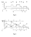
- a plot 39 of the number of requests waiting to be processed by a processing system is shown.
- the plot shows periods 40 1 , 40 2 when the system is busy and a period 41 when the system is idle.
- the plot 42 includes lines 42 1 , 42 2 , 42 3 , 42 4 representing a time a request will wait in the system before departure.
- a new arrival is represented by a jump of magnitude b j .
- a sequence of waiting, inter-departure times and idle times can be determined.
- Equations 18 and 20 can be presented in a similar format.
- the ⁇ operation involves integrating the probability distribution function W ( t ) ⁇ C ( t ) for negative variate values (for example, over the range - ⁇ 0) so as to find a weighting ⁇ and replacing this part of the probability distribution function with a delta function at zero variate value, the delta function having pre-weighting ⁇ .
- the ⁇ operation involves integrating the probability distribution function W ( t ) ⁇ C ( t ) for positive variate values so as to find a weighting ⁇ and replacing this part of the probability distribution function with a delta function at zero variate value, the delta function having pre-weighting ⁇ .
- the negative part of the probability distribution function is flipped by reflecting the function about the y-axis.
- probability distribution functions W, D, I for waiting, inter-departure times and idle times can be determined.
- the computer system 2 ( Figure 2) can thus be used to simulate the processing system and obtain probability distributions functions for waiting, inter-departure times and idle times.
- the system and process hereinbefore described may be used to simulate any system which is driven by randomness.
- the process has the advantage that they can be used to simulate a wider class of stochastic models than existing analytical methods and are more accurate and faster at computing models than using Monte Carlo methods.
Landscapes
- Engineering & Computer Science (AREA)
- Physics & Mathematics (AREA)
- Data Mining & Analysis (AREA)
- General Physics & Mathematics (AREA)
- Mathematical Optimization (AREA)
- Pure & Applied Mathematics (AREA)
- Theoretical Computer Science (AREA)
- Mathematical Physics (AREA)
- Computational Mathematics (AREA)
- Mathematical Analysis (AREA)
- Life Sciences & Earth Sciences (AREA)
- Operations Research (AREA)
- Probability & Statistics with Applications (AREA)
- Bioinformatics & Cheminformatics (AREA)
- Algebra (AREA)
- Evolutionary Biology (AREA)
- Databases & Information Systems (AREA)
- Software Systems (AREA)
- General Engineering & Computer Science (AREA)
- Bioinformatics & Computational Biology (AREA)
- Complex Calculations (AREA)
Abstract
Description
- The present invention relates to a computer system for simulating a physical system.
- In a clinical trial, an experimenter administers a fixed dose of a drug to several patients and monitors the concentration of the drug in the blood stream as a function of time. The clinical trial can be simulated as a model using a computer system to determine whether the concentration of the drug exceeds a therapeutic level, but falls below a harmful level.
- The model may depend on several factors such as the rate at which the drug passes from the stomach to the blood stream and the rate at which it is excreted. These rates vary from person to person. Moreover, concentration depends on the volume of distribution, which in turn depends upon body weight. The model uses probability distribution functions of rates and weights. However, due to the possible high number of distributions and their complexity, plentiful computational resources are needed to model the trial. Otherwise it can take a long time to simulate the trial. In fact, this problem is common in simulating physical systems.
- The present invention seeks to provide an improved computer system in which a physical system can be simulated more quickly and/or with less processing power, while maintaining accuracy.
- According to a first aspect of the present invention there is provided a computer system for simulating a physical system comprising a first module configured to convert a probability distribution function of a physical property into a discrete function having at least one segment and a second module configured to perform an exact transformation of each segment.
- The second module may be configured to add results of each transformation to provide a new probability distribution function. The second module may be configured to perform a unary transformation of each segment. The second module may be configured to perform a binary transformation of each segment with each segment of another discrete probability distribution function, such as convolution of each segment with each segment of another discrete probability distribution function and/or addition, subtraction, multiplication or division integral transformation of each segment with each segment of the other discrete function.
- The probability distribution function may be of an amount of a drug or a time interval in a processing system.
- According to a second aspect of the present invention there is provided a method of simulating a physical system, the method comprising converting a probability distribution function of a physical property into a discrete function having at least one segment and performing an exact transformation of each segment.
- According to a third aspect of the present invention there is provided a computer program comprising instructions for performing the method.
- According to a fourth aspect of the present invention there is provided a computer program product comprising a computer-readable medium storing a computer program for causing a computer to convert a probability distribution function of a physical property into a discrete function having at least one segment and to perform an exact transformation of each segment.
- Embodiments of the present invention will now be described, by way of example, with reference to the accompanying drawings in which:
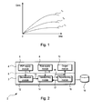
- Figure 1 are illustrative plots of concentration of a drug in the blood stream as a function of time;
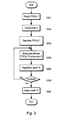
- Figure 2 is a schematic block diagram of a computer system for simulating a physical system in accordance with the present invention;
- Figure 3 is a process flow diagram of a simulating process performed by the computer system shown in Figure 2;
- Figures 4a to 4d illustrate, for a simple example, results of performing steps in the simulating process shown in Figure 3;
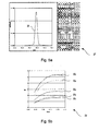
- Figures 5a and 5b illustrate, for another example, results of the simulating process shown in Figure 3;
- Figure 6 illustrates a unary transformation;
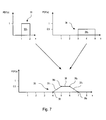
- Figure 7 illustrates a binary transformation;
- Figure 8 is a plot of number of requests in a processing system which can be modelled in accordance with the present invention; and
- Figure 9 is a plot of waiting time of the requests shown in Figure 8.
- Drug companies usually formulate a drug such that when it is administered to a patient its concentration, for example in the blood stream, exceeds a level at which it provides a therapeutic effect, but falls short of a harmful level. However, the effect of the drug will vary from person to person, for example due to differences in their body weights. Thus, drug companies usually formulate the drug to have a dose such that the concentration falls within these levels when taken by most of the population. The size of dose is usually found as part of a clinical trial.
- For example, referring to Figure 1, if a fixed dose of a drug is administered to three different patients, then the concentration of the drug in their respective blood streams could vary with time as shown in
plots - Before conducting any trial, an experimenter may wish to ascertain ranges of doses which are safe to use. Furthermore, during the trial, the experimenter may wish to check that the results of the trial are as expected. For this reason, the experimenter simulates the concentration of the drug in the blood stream based on an understanding of how the body processes the drug.
- Referring to Figure 2, a
computer system 2 for simulating a physical system, such as concentration of a drug in the blood stream, is shown. Thecomputer system 2 may be distributed and, thus, may include aclient 3 andserver 4 connected via anetwork 5. Theclient 3 may be a relatively low-specification personal computer, whereas theserver 4 can be a high performance computer. Alternatively, thecomputer system 2 may be implemented in a single computer. - The
computer system 2 includes amodule 6 for supplying at least one inputprobability distribution function 7, amodule 8 for supplying at least onerule 9 for processing the at least one inputprobability distribution function 7 and amodule 10 for outputting and post-processing at least one outputprobability distribution function 11. Thesemodules client 3. - Each
probability distribution function 7 defines a variable or a parameter of a physical system, such as body weight. - The probability distribution function(s) 7 and
rules 9 may be prepared manually by the user and/or selected from a pre-stored database. - The
computer system 2 further includes afirst module 12 for converting the at least one inputprobability distribution function 7, if not already discrete, into corresponding discrete probability distribution function(s) 13, amodule 14 for performing an exact probabilistic transformation of the discrete probability distribution function(s) 14 so as to provide at least one transformed probability distribution function 15 (herein also referred to as the "result") and a second module for converting theresult 15 into at least onediscrete result 17. - The
first discretising module 12 can take aprobability distribution function 7, such as f(x), and divide at least part of thefunction 7 over an interval (X1→X2) into several segments over a plurality of intervals (x1→x1,1, x1,1→x1,2, ..., and x1,n→x2). Thediscretising module 13 approximates theprobability distribution function 7 in each or, if there is only one, the segment and may ensure that the sum of the areas of the segments equals one. However, thediscretising module 12 can simply approximate theprobability distribution function 7 over the interval, such that there is a single segment. - The
discretising module 12 divides theprobability distribution function 7 according to the rate of change of theprobability distribution function 7 so as to provide higher resolution when theprobability distribution function 7 changes rapidly and lower resolution when theprobability distribution function 7 changes slowly. However, thediscretising module 12 can divide theprobability distribution function 7 into equidistant intervals or equiprobable intervals. The number of segments can be chosen to provide a given degree of accuracy. Typically, the number of segments is of theorder 1 to 10,000. However, the number of segments can be higher. - The
discretising module 12 approximates theprobability distribution function 7 in each interval as a uniform probability distribution. Thus, the discrete, approximateprobability distribution function 13 resembles a histogram or bar chart. However, other probability distributions, such as non-uniform linear or quadratic probability distribution functions, may be used provided they can be exactly (e.g. analytically) transformed. - The
transformation module 14 may perform unary transformations, such as square root or cosine, of a function or binary transformations, such addition, subtraction, multiplication or division integral transforms, of the probability distribution function(s) 7. Other transformations are possible. Furthermore, one or more unary and one or more binary transformations may be combined, for example sequentially. - The
transformation module 14 is able to perform (or perform more easily) an exact, for example analytical, probabilistic transformation because thediscretising module 12 has converted eachprobability distribution function 7 into discrete, uniformly valued segments. - The second discretising module 16 (hereinafter referred to as the "
repartitioning module 16") takes what may be acontinuous result 15 and converts it into adiscrete result 17 which can be fed back intotransformation module 14 and/or output. - The
computer system 2 may be provided with anoptional database 18 for storingprobability distribution functions rules 9 andresults - The
computer system 2 includes at least one processor (not shown), memory (not shown) storing software for providing themodules - Referring to Figure 3, a process flow diagram of a process of a method of simulating a physical system in accordance with the present invention is shown.
- Referring also to Figure 4a, the process will be described using simple
probability distribution functions - The
probability distribution functions 7 andrules 9 are specified by a user and supplied by the probability distribution function-supplying module 6 (Figure 2) and rule-supplying module 8 (Figure 2) to the discretising module 12 (Figure 2) and transformation modules 14 (Figure 2) respectively (steps S301 & S302). - A first
probability distribution function 71 is a uniform function over afirst interval 20. A secondprobability distribution function 72 is an exponential function. - The discretising module 12 (Figure 2) divides an
interval 21 of the secondprobability distribution function 72 into first andsecond intervals probability distribution function 72 in eachinterval - In this example, the
rule 9 is to convolve the first and secondprobability distribution functions 
- Referring to Figure 4b, the transformation module 14 (Figure 2) applies the
rule 9 to produce a result 15 (Figure 2), which in this example involves transformation module 14 (Figure 2) convolvingprobability distribution function 71 with the segments 221, 222 producingpartial solutions - Referring to Figure 4c, a comparison of the
cumulative result 23 and a full, conventionalanalytical result 24 is shown. It will be appreciated that this comparison is for the purposes of illustration only and that thecomputer system 2 does not usually carry out a full, conventional analytical solution not least because the solution is impossible or onerous to compute. - The repartition module 16 (Figure 2) may convert the result 15 (Figure 2), in this case
cumulative result 23, into a discretised result 17 (Figure 2) (step S305). - Referring to Figure 4d, the repartition module 16 (Figure 2) may divide the
cumulative result 23 into intervals 251, 252, 253 and approximate thecumulative result 23 in these intervals 251, 252, 253 as approximations 261, 262, 263. - The process may continue to process the result 15 (step S306 & S303). For example, the transformation module 14 (Figure 2) may perform further transformations on approximations 261, 262, 263.
- The results may be output to the output module 10 (Figure 2) for displaying and post-processing by the user (step S306). Post-processing may include determining quantiles, determining mean and variance and/or determining area under the curve.
- As mentioned earlier, the computer system 2 (Figure 2) can simulate the concentration of the drug in the blood stream.
- The concentration, C, is the amount of drug in the blood stream, B, divided by the so-called "volume of distribution", V, i.e.

- For a single individual, the volume is given:

where Wi is the body weight of the individual and ki is a person-specific constant. Thus, the concentration for the individual i is:
- For an individual, B , ki , Wi are single numbers and so it is easy to decide whether Ci falls between a therapeutic level T and a harmful level H.
- For a population, however, it is harder to decide whether the concentration Ci falls with these limits. Within a population, body weight has a probability density PDF(W) and constant also has a probability density PDF(k). Thus, for a given dose, not all individuals will have the same concentration Ci . Even if the mean concentration 〈Ci 〉 lies within limits, the concentration for some individuals may fall below the therapeutic level T or exceed the harmful level H. By calculating PDF(C), the experimenter can assess the efficacy of the clinical trial.
- To simulate the concentration of the drug in the blood stream, the probability distribution function module 6 (Figure 2) supplies the following probability distribution functions 7 (Figure 2) to the discretising module 12 (Figure 2):





where Ve is the random variation in the volume of distribution, w is body weight, d is the amount of drug in the stomach, b is the amount of drug in the blood stream, e is the amount of drug in the kidneys (i.e. excreted), k 1 is the decay constant for the drug passing from the stomach to the blood stream and k 2 is the decay constant for the drug passing from the blood stream to the kidneys. - In equations 5a to 5f above, two distributions are used, namely normal(µ ,σ2) which is the normal distribution P(x) in a variate x having mean µ and standard deviation σ2 and defined by:

and uniform (a,b) which is the uniform distribution function defined by:
- The discretising module 12 (Figure 2) converts the normal
probability distribution functions 7 into discrete functions having, for example, three segments (not shown). - The rule-supplying module 8 (Figure 2) supplies a function, namely:

where 0.21 is phenomenological constant. - The rule-supplying module 8 (Figure 2) also supplies differential equations, namely:


- The transformation module 14 (Figure 2) applies the rules found in
equations 8 and 9a to 9c, to the discretised probability distribution functions based on equations 5a to 5e. - Different output may be selected. For example, PDF(d), PDF(b) or PDF(e) can be selected at different times t, for example t = 0.2, 0.4, 0.6, 0.8, 1.0 and 1.2.
- Referring to Figure 5a, a screen shot 27 of an output provided through the output module 10 (Figure 2) is shown. The screen shot 27 shows a
plot 28 of PDF(b) at t = 1.0. - Referring to Figure 5b, a screen shot 28 of another output provided through the output module 10 (Figure 2) is shown. The screen shot 29 shows plots 301, 302, 303, 304, 305 of C = blV with time t. The plots 301, 302, 303, 304, 305 include not only a plot 303 of medium concentration, but also quantile plots.
- As explained earlier, the transformation module 14 (Figure 2) is able to perform an exact probabilistic transformation because the discretising module 12 (Figure 2) has converted each
probability distribution function 7 into discrete, uniformly valued segments. - Some examples of exact unary and binary transformations of discrete probability distribution functions will now be described in more detail.
- Referring to Figure 6, an example of a discrete
probability distribution function 31 is shown. The discreteprobability distribution function 31 may correspond to a discrete probability distribution function 13 (Figure 2) produced by the discretisation module 12 (Figure 2). - The
probability distribution function 31 has threesegments - A unary transformation of the discrete
probability distribution function 31 is carried out by transforming each segment separately 311, 312, 313. A square root transformation will be used to illustrate a unary transformation: - The transformation module 14 (Figure 2) takes the square root of the starting variate value 321 (x 1) of the
first segment 311 to produce a new starting variate value
first segment 311 to produce a new finishing variate value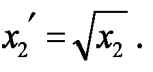

second segment 312 and so on. - Referring to Figure 7, further examples of discrete
probability distribution functions probability distribution functions - A first
probability distribution function 33 has onesegment 331 having variate starting and finishing values of (xA, xB ), in this case (1, 2), and probability distribution value c, in thiscase 1. A secondprobability distribution function 34 has onesegment 341 having variate starting and finishing values of (xC, xD ), in this case (3, 5), and probability distribution value j, in this case 0.5. - A binary transformation of the discrete
probability distribution functions probability distribution function 35. An addition integral transformation of the discreteprobability distribution functions - The transformation module 14 (Figure 2) determines a starting variate value 361 of the transformed
probability distribution function 35 by adding the start variate values of thefunctions probability distribution function 35 rises up a first slope 371 to a first shoulder variate value 362. The transformation module 14 (Figure 2) may determine the first shoulder variate value 362 using, for example:
- The transformed
probability distribution function 35 may have aplateau 38, although it need not necessarily do so. The transformation module 14 (Figure 2) may determine a second shoulder variate value 363 using, for example:
- The transformed
probability distribution function 35 drops down a second slope 372 to a finishing variate value 364. The transformation module 14 (Figure 2) determines the finishing variate value 364 by adding the finishing variate values of thefunctions - If the first and second discrete
probability distribution functions probability distribution function 33 with a first segment from the secondprobability distribution function 34, the first segment from the firstprobability distribution function 33 with a second segment from the secondprobability distribution function 34 and so on until the first segment from the firstprobability distribution function 33 with a last segment from the secondprobability distribution function 34 then a second segment from the firstprobability distribution function 33, with the first segment from the secondprobability distribution function 34 and so on. - For an addition integral transformation, the slopes 371, 372 are linear. For other forms of integral transformation, the slopes 371, 372 may have other shapes, such as logarithmic. The
plateau 38 need not have a constant value, but may have, for example in the case of multiplication integral transformation, a logarithmic shape. - The system and process hereinbefore described may be used to simulate any system which is driven by randomness, such as queuing or manufacturing processes.
- For example, the system may be a computer system (hereinafter referred to as a "processing system"), in which requests are processed using a First-In-First-Out (FIFO) arrangement.
- A request j arrives at a system time tj. If the system is busy, then the request waits for a time wj. The system services the request in time bj, after which a result leaves the system at time rj . The time span between arrivals j-1 and j may be denoted αj and the time span between departures j-1 and j may be denoted dj . The time span for which the system is idle before the arrival of request j may be denoted ij .
- Individual events and distributions of event are listed in Table 1 below:
Table 1 Individual events Distribution of events tj arrival time - - wj waiting time W distribution of waiting times bj service time B distribution of service times rj departure time - - αj inter-arrival time A distribution of inter-arrival times dj inter-departure time D distribution of inter-departure times ij idle time I distribution of idle times - Referring to Figure 8, a
plot 39 of the number of requests waiting to be processed by a processing system is shown. The plot shows periods 401, 402 when the system is busy and aperiod 41 when the system is idle. - Referring to Figure 9, a
plot 42 of waiting time is shown. Theplot 42 includeslines - If the system has been idle (as for j = 1 and j = 4), then the remaining service time for the request immediately starts to decrease. However, if the system has been busy (as for j = 2 and j = 3), then a newly-arrived request is subject to a waiting time which equals the sum of the service times of previous requests.
- Thus, the following relations hold:


and therefore

and a so-called "breathing space" can be defined as:
such thatequation 13 can be re-written as
and

- For a given sequence of inter-arrival times and service times, a sequence of waiting, inter-departure times and idle times can be determined.
-
Equations 



where π and π̅ are sweeping operations for maximum and minimum respectively and where equation 19 can be presented as:
-
Equations - The π operation involves integrating the probability distribution function W(t) ⊕C(t) for negative variate values (for example, over the range -∞→0) so as to find a weighting α and replacing this part of the probability distribution function with a delta function at zero variate value, the delta function having pre-weighting α.
- The π̅ operation involves integrating the probability distribution function W(t) ⊕ C(t) for positive variate values so as to find a weighting β and replacing this part of the probability distribution function with a delta function at zero variate value, the delta function having pre-weighting β. The negative part of the probability distribution function is flipped by reflecting the function about the y-axis.
- The waiting time probability distribution function W is determined self consistently. This may involve guessing an initial waiting time probability distribution function W, such as there is no waiting, and iteratively calculating
equation 18 until the result converges. For example, this may involve determining whether two results are the same, i.e. Wi = W i-1, or any difference is small, for example based on chisquared test. Once the waiting time probability distribution function W has been determined, the inter-departure times and idle times probability distribution functions D, I can be determined. - Thus, for a given inter-arrival time probability distribution function A and a service time probability distribution function B, probability distribution functions W, D, I for waiting, inter-departure times and idle times can be determined.
- The computer system 2 (Figure 2) can thus be used to simulate the processing system and obtain probability distributions functions for waiting, inter-departure times and idle times.
- The system and process hereinbefore described may be used to simulate any system which is driven by randomness. The process has the advantage that they can be used to simulate a wider class of stochastic models than existing analytical methods and are more accurate and faster at computing models than using Monte Carlo methods.
Claims (11)
- A computer system for simulating a physical system comprising:a first module (12) configured to convert a probability distribution function (7) of a physical property into a discrete function having at least one segment; anda second module (14) configured to perform an exact transformation of each segment.
- A computer system according to claim 1, wherein the second module (14) is configured to add results of each transformation to provide a new probability distribution function.
- A computer system according to claim 1 or 2, wherein the second module (14) is configured to perform a unary transformation of each segment.
- A computer system according to claim 3, wherein the second module (14) is configured to perform a binary transformation of each segment with each segment of another discrete probability distribution function.
- A computer system according to claim 4, wherein the binary transformation comprises convolution of each segment with each segment of another discrete probability distribution function.
- A computer system according to claim 4 or 5, wherein the binary transformation comprises addition, subtraction, multiplication or division integral transformation of each segment with each segment of another discrete probability distribution function.
- A computer system according to any preceding claim, wherein the probability distribution function is of an amount of a drug.
- A computer system according to any preceding claim, wherein the probability distribution function is of a time interval in a processing system.
- A method of simulating a physical system comprising:converting a probability distribution function (7) of a physical property into a discrete function having at least one segment; andperforming an exact transformation of each segment.
- A computer program comprising instructions for performing a method according to claim 9.
- A computer program product comprising a computer-readable medium storing a computer program for causing a computer to convert a probability distribution function of a physical property into a discrete function having at least one segment and to perform an exact transformation of each segment.
Priority Applications (2)
| Application Number | Priority Date | Filing Date | Title |
|---|---|---|---|
| EP05111457A EP1791064A1 (en) | 2005-11-29 | 2005-11-29 | Computer system for simulating a physical system |
| US11/604,819 US20070124123A1 (en) | 2005-11-29 | 2006-11-28 | Computer system for simulating a physical system |
Applications Claiming Priority (1)
| Application Number | Priority Date | Filing Date | Title |
|---|---|---|---|
| EP05111457A EP1791064A1 (en) | 2005-11-29 | 2005-11-29 | Computer system for simulating a physical system |
Publications (1)
| Publication Number | Publication Date |
|---|---|
| EP1791064A1 true EP1791064A1 (en) | 2007-05-30 |
Family
ID=37056736
Family Applications (1)
| Application Number | Title | Priority Date | Filing Date |
|---|---|---|---|
| EP05111457A Withdrawn EP1791064A1 (en) | 2005-11-29 | 2005-11-29 | Computer system for simulating a physical system |
Country Status (2)
| Country | Link |
|---|---|
| US (1) | US20070124123A1 (en) |
| EP (1) | EP1791064A1 (en) |
Family Cites Families (2)
| Publication number | Priority date | Publication date | Assignee | Title |
|---|---|---|---|---|
| FI113410B (en) * | 2002-05-31 | 2004-04-15 | Ekahau Oy | Probalistic model for positioning technique |
| WO2006084196A2 (en) * | 2005-02-04 | 2006-08-10 | Entelos, Inc. | Method for defining virtual patient populations |
-
2005
- 2005-11-29 EP EP05111457A patent/EP1791064A1/en not_active Withdrawn
-
2006
- 2006-11-28 US US11/604,819 patent/US20070124123A1/en not_active Abandoned
Non-Patent Citations (5)
| Title |
|---|
| BERLEANT D: "Automatically verified reasoning with both intervals and probability density functions", INTERVAL COMPUTATIONS, no. 2, 1993, XP002403054, Retrieved from the Internet <URL:http://class.ee.iastate.edu/berleant/home/me/cv/papers/pdfs93.ps> [retrieved on 20061011] * |
| CARRERAS C ET AL: "Grid-based histogram arithmetic for the probabilistic analysis of functions", PROCEEDINGS OF THE 4TH INTERNATIONAL SYMPOSIUM ON ABSTRACTION, REFORMULATION, AND APPROXIMATION, LECTURE NOTES IN COMPUTER SCIENCE, vol. 1864, 2000, Springer Verlag, London, UK, pages 107 - 123, XP002403055, ISBN: 3-540-67839-5 * |
| COLOMBO A G ET AL: "A powerful numerical method to combine random variables", IEEE TRANSACTIONS OF RELIABILITY, vol. R-29, no. 2, June 1980 (1980-06-01), pages 126 - 129, XP008069981 * |
| KAPLAN S: "On the method of discrete probability distributions in risk and reliability calculations - Applications to seismic assessment", RISK ANALYSIS, vol. 1, no. 3, 1981, pages 189 - 196, XP008069972 * |
| S. KAPLAN: "On The Method of Discrete Probability Distribution in Risk and Reliability Calculations - Application to Seismic Risk Assessment", RISK ANALYSIS, vol. 1, 1981, pages 189 |
Also Published As
| Publication number | Publication date |
|---|---|
| US20070124123A1 (en) | 2007-05-31 |
Similar Documents
| Publication | Publication Date | Title |
|---|---|---|
| US12051487B2 (en) | Systems and methods for supplementing data with generative models | |
| Warrens | Some paradoxical results for the quadratically weighted kappa | |
| US8793144B2 (en) | Treatment effect prediction system, a treatment effect prediction method, and a computer program product thereof | |
| US8073629B2 (en) | Simulation system of function of biological organ | |
| US20050288910A1 (en) | Generation of continuous mathematical model for common features of a subject group | |
| US10380506B2 (en) | Generation of occupant activities based on recorded occupant behavior | |
| Van Hest et al. | Estimating infectious diseases incidence: validity of capture–recapture analysis and truncated models for incomplete count data | |
| US20030025696A1 (en) | Method and system for generating a graphical representation | |
| CN115966314B (en) | Data processing method and device, electronic equipment and storage medium | |
| EP3742453A1 (en) | Computer-implemented method for classifying a patient based on codes of at least one predetermined patient classification and computerized system to carry it out | |
| EP1791064A1 (en) | Computer system for simulating a physical system | |
| DasGupta | Normal approximations and the central limit theorem | |
| Rathnayake et al. | Tolerance bands for functional data | |
| Balakrishnan et al. | Semi-parametric likelihood inference for Birnbaum–Saunders frailty model | |
| Jensema | An application of latent trait mental test theory | |
| CN118213088B (en) | Rare disease clinical trial sample content estimation method and system | |
| Lee et al. | Estimation and reduction of bias in self‐controlled case series with non‐rare event dependent outcomes and heterogeneous populations | |
| Yafune et al. | Bootstrap approach for constructing confidence intervals for population pharmacokinetic parameters. II: A bootstrap modification of standard two‐stage (STS) method for phase I trial | |
| Bailey | Application of stochastic epidemic modelling in the public health control of HIV/AIDS | |
| Martin et al. | A model for the optimal control of a measles epidemic | |
| CN120448609B (en) | A data visualization method and system for influenza vaccine clinical trials | |
| Rice et al. | Approximate maximum likelihood estimation in cure models using aggregated data, with application to HPV vaccine completion | |
| Cummings | Adjusting standard errors and confidence intervals | |
| Kaskasamkul et al. | Confidence Intervals using Bootstrap Methods for the Parameter of the zero-truncated Poisson-Shanker Distribution and their Application | |
| Rapoport | Directions in Mathematical Psychology, I |
Legal Events
| Date | Code | Title | Description |
|---|---|---|---|
| PUAI | Public reference made under article 153(3) epc to a published international application that has entered the european phase |
Free format text: ORIGINAL CODE: 0009012 |
|
| AK | Designated contracting states |
Kind code of ref document: A1 Designated state(s): AT BE BG CH CY CZ DE DK EE ES FI FR GB GR HU IE IS IT LI LT LU LV MC NL PL PT RO SE SI SK TR |
|
| AX | Request for extension of the european patent |
Extension state: AL BA HR MK YU |
|
| 17P | Request for examination filed |
Effective date: 20070620 |
|
| 17Q | First examination report despatched |
Effective date: 20070717 |
|
| AKX | Designation fees paid |
Designated state(s): DE GB |
|
| STAA | Information on the status of an ep patent application or granted ep patent |
Free format text: STATUS: THE APPLICATION IS DEEMED TO BE WITHDRAWN |
|
| 18D | Application deemed to be withdrawn |
Effective date: 20090603 |