EP1626596A1 - System and method for wireless coverage detection - Google Patents
System and method for wireless coverage detection Download PDFInfo
- Publication number
- EP1626596A1 EP1626596A1 EP05252866A EP05252866A EP1626596A1 EP 1626596 A1 EP1626596 A1 EP 1626596A1 EP 05252866 A EP05252866 A EP 05252866A EP 05252866 A EP05252866 A EP 05252866A EP 1626596 A1 EP1626596 A1 EP 1626596A1
- Authority
- EP
- European Patent Office
- Prior art keywords
- cells
- locations
- mobile device
- time
- region
- Prior art date
- Legal status (The legal status is an assumption and is not a legal conclusion. Google has not performed a legal analysis and makes no representation as to the accuracy of the status listed.)
- Withdrawn
Links
- 238000000034 method Methods 0.000 title claims abstract description 80
- 238000001514 detection method Methods 0.000 title description 2
- 238000003860 storage Methods 0.000 abstract description 3
- 210000004027 cell Anatomy 0.000 description 74
- 230000008569 process Effects 0.000 description 47
- 238000012360 testing method Methods 0.000 description 10
- 230000001413 cellular effect Effects 0.000 description 9
- 210000003888 boundary cell Anatomy 0.000 description 3
- 238000004891 communication Methods 0.000 description 3
- 238000004519 manufacturing process Methods 0.000 description 3
- 239000000203 mixture Substances 0.000 description 3
- 230000008901 benefit Effects 0.000 description 2
- 230000006870 function Effects 0.000 description 2
- 238000005259 measurement Methods 0.000 description 2
- 230000000737 periodic effect Effects 0.000 description 2
- 238000005303 weighing Methods 0.000 description 2
- 230000004075 alteration Effects 0.000 description 1
- 230000006399 behavior Effects 0.000 description 1
- 230000005540 biological transmission Effects 0.000 description 1
- 230000008602 contraction Effects 0.000 description 1
- 238000012937 correction Methods 0.000 description 1
- 238000013461 design Methods 0.000 description 1
- 230000000694 effects Effects 0.000 description 1
- 229920001690 polydopamine Polymers 0.000 description 1
- 238000012545 processing Methods 0.000 description 1
- 238000007670 refining Methods 0.000 description 1
- 238000005070 sampling Methods 0.000 description 1
- 238000000638 solvent extraction Methods 0.000 description 1
- 238000006467 substitution reaction Methods 0.000 description 1
- 238000012546 transfer Methods 0.000 description 1
- 230000001960 triggered effect Effects 0.000 description 1
Images



Classifications
-
- H—ELECTRICITY
- H04—ELECTRIC COMMUNICATION TECHNIQUE
- H04W—WIRELESS COMMUNICATION NETWORKS
- H04W24/00—Supervisory, monitoring or testing arrangements
- H04W24/08—Testing, supervising or monitoring using real traffic
-
- H—ELECTRICITY
- H04—ELECTRIC COMMUNICATION TECHNIQUE
- H04W—WIRELESS COMMUNICATION NETWORKS
- H04W24/00—Supervisory, monitoring or testing arrangements
-
- H—ELECTRICITY
- H04—ELECTRIC COMMUNICATION TECHNIQUE
- H04W—WIRELESS COMMUNICATION NETWORKS
- H04W16/00—Network planning, e.g. coverage or traffic planning tools; Network deployment, e.g. resource partitioning or cells structures
- H04W16/18—Network planning tools
Definitions
- This disclosure relates to wireless coverage detection and more particularly to systems and methods for using mobile devices for detecting the boundary of a measurable phenomenon, such as the signal quality of RF broadcasts.
- RF field is undersampled in time, since each sample covers only a fraction of a second per month at any one location.
- Another disadvantage of drive testing is that the RF field is also undersampled in space, because most of the major roads are not driven their entire length and only some of the minor roads are driven. Drive testing misses all locations without a road, such as parks, stadiums, homes, offices, conference centers, etc.
- a system and method for determining the spatial boundary of measurable phenomenon such as the quality of a broadcast signal at various locations within geographical areas covered by the broadcast signal.
- Data representing relative signal quality at various locations within the geographical area is created within a mobile device, such as a cell phone capable of receiving the broadcast signals.
- the data is stored, and refined, within the device so as to define weak signal quality areas within at least a portion of the geographical area traveled by the mobile device.
- the data stored within the mobile device is from time to time communicated to the central broadcast system.
- the refinement of the data in the device allows for long storage periods so that signal quality can be reported over long time spans. By collecting such data from a plurality of such devices, the central system can map the signal strength over the entire geographical area.
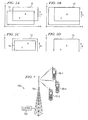
- FIGURE 1A shows geographical areas defined by a mobile device
- FIGURES 1B, 1C, and 1D show movement, expansion and contraction of the geographical area of FIGURE 1;
- FIGURES 2, 3, and 4 show flow charts of one embodiment of system operations
- FIGURE 5 shows one embodiment of a mobile device
- FIGURES 6A, 6B, 5C, 6D and 6E show one embodiment of the steps for changing the size of cells.
- FIGURE 7 shows one embodiment of a cellular system using the systems and methods described herein.
- FIGURE 1A shows geographical area I 1 where the user of a mobile device (for example, a cellular telephone) spends most of his/her time.
- the letter 'A' is positioned at the center of geographical area 11. For discussion purposes, this is called the 'home' region and in discussing FIGURES 1A-1D the method discussed with respect to FIGURE 2 will be used.
- FIGURE 1B shows the expanded region 13.
- the new home region has expanded on the north and east.
- the expansion amount could be by just enough to include the user's new location or could be by an integral number of bins (cells), or by doubling the original size, etc.
- FIGURE 1C shows an example where the user remains within the confines of region 12 and, periodically, as will be discussed hereinafter, the region is reduced.
- acts performed periodically can be performed at regular intervals or at random intervals.
- region 12 is reduced on all sides to form region 14.
- FIGURE 1D shows that the home region, now region 15, has again been expanded on the north and east to include areas of user movement.
- the home region now includes the new areas of user movement, and omits the areas where the user no longer goes.
- the home region has effectively moved to follow the user from A to B.
- the coordinates (and the data associated with the coordinates) are cached (home coordinate cache) and a new temporary region is created.
- the system periodically increments a count associated with the region the user is currently in and periodically deletes from the cache the region with the smallest count.
- the system has established a home region.
- the system establishes which cached region is the user's home region. There may be a tie, or a near-tie, for first place, depending on the usage pattern. However, this does not matter since the important thing is to choose a region where the user spends a lot of time.
- it takes four numbers to store the bin information.
- the numbers may be, for example, latitude/longitude, or distance (in bins, or some other unit) plus an angle from a known tower, or some other coordinate system (which need not be Cartesian).
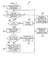
- FIGURE 2 shows one embodiment of a flowchart showing system and method 20 for determining the home region for storing data pertaining to signal strength.
- Process 201 starts with an initial home region.
- One embodiment for determining the home region is shown in FIGURE 3 to be discussed hereinafter.
- Process 202 determines whether the user has moved outside of the home region. If the user has moved outside the home region, process 203 determines if the user has moved beyond a given distance. If not, then the boundary is expanded via process 204 as discussed above. If the user has moved beyond a given distance, then the prior region's data is stored in a cache via process 205. Process 206 then determines if the new location is in cache. If so, that cached region becomes the new home region. If not, then process 208 creates a new home region.
- Process 209 periodically increments the count for the current region and process 210 periodically shrinks the current region. Either or both of these actions can be incremented periodically, such as every minute (hour), (day), etc., as desired. While uniform shrinking is discussed, an important factor is that shrinkage (whether uniform or nonuniform) is unbiased over the long run. Thus, the shrinkage need not be uniform across the region, and one side could be reduced at one time and a different side reduced at another time. The side or sides to be reduced could be determined in order (north, south, east, west, etc.) or in random order, and any number of sides can be reduced at a time.
- this system will continually refine itself so that if a user has moved to a new home region, the new home region will soon become the official home region and the system will continue without anything being done by either the user or the central system to which the device will eventually report.
- the size of the area will continually refine downward (or upward) so that as the user's movements reduce (or increase) the home region also reduces (or increases).
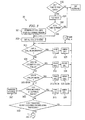
- FIGURE 3 shows one embodiment 30 of a system and method for constructing a grid of cells describing the measurement of the phenomenon, for example, quality of wireless coverage.
- Process 301 constructs a cell grid over the region where the user presently is located. This cell grid can be as fine as memory will allow. Note that the memory can be different for different mobile devices, and thus, the size of grid area or the refinement therein can be different.
- Process 302 sets all cells to 0 initially.
- Processes 303 to 306 are several examples of a defined "bad" cell. In this context "bad" can be defined in any manner subjectively observable by the device and generally pertains to the quality of the signal. No signal is the ultimate bad quality.
- a dropped call is one example of a "bad" reading. If desired, bad readings can be graded such that a dropped call can be, say, the equivalent of two low RF signal readings, while other factors only give rise to a single incremented count.
- Process 303 determines if a call has been dropped. If so, process 313 determines the cell where the dropped call occurred and an incremented count is made in that cell via process 323. As discussed, this increment would be, for example, a 1 added to the cell to show that a call has been dropped in that cell by this device. Again, note that this information is maintained in the device itself, and is not, at this point, communicated to the central system.
- Process 304 determines whether an attempted call has failed, if it has, process 314 finds which cell the call was attempted from. That cell is incremented via process 324.
- Process 305 to 305N checks for other failure modes and the proper cells are located and incremented via processes 315 to 315N and 325 to 325N.
- Process 306 checks to see if a periodic check of strength has failed, and if so, then process 316 finds which cell the signal strength has failed in and process 326 increments that cell.
- Process 306 works under periodic control of process 307 and can, if desired, be under random control, or triggered by external signals or any other manner desired.
- Process 308 determines whether a triggering event for reducing the region has occurred. If it has, then system and method 40, shown in FIGURE 4 is entered and, as will be discussed in more detail hereinafter, operates to reduce the memory required for the active region so that more data can be stored for faulty cells.
- Process 330 determines if it is time to file the data with the central system. If it is, then data, via process 331, is transferred from the cell phone to the central system. This transfer can occur periodically, randomly, or on command from the central system as will be discussed, this time can be once a year, or every several months, or sooner as desired. At some point in time, it may be proper to reset the cells to 0. If so, then the system triggers process 302 and system and method 30 will repeat.
- FIGURE 4 shows one embodiment 40 of a system and method for refining the boundary of the region of poor coverage, by giving cells not on the boundary coarse granularity, and cells on the boundary fine granularity.
- Processes 401-402 control coarse granularity with respect to adjacent cells which have approximately equal density of counts per unit area. These approximately equal cells are merged into a single cell, and the cell's count is set equal to the sum of the counts of the merged cells. Note that this process frees up memory, which is used in later steps.
- any reasonable interpretation of 'equal' will work - exactly equal, within "n” counts/area, within “n” percent, etc.
- a user can decide how to design the system and method to take into account the desired interpretation of "all cells are equal”: (i.e.) the difference between neighbors is small, the difference between max and min is small, the difference between max and average is small, etc.
- any method can be chosen, but it is good practice to use the difference between max and min; otherwise the method could be fooled by a smooth gradient.
- Processes 403-406 control fine granularity.
- Process 403 divides each cell whose density is not "equal" to that of its neighbors into four cells. This uses the memory which was freed in the previous step. If there is not enough memory, as determined by process 404 to do this step, then division is ended as shown in process 403.
- Process 406 assigns a count to each new cell created in process 403.
- the count is chosen as follows. Assume the original cell's count is C.
- FIGURE 5 shows one example of a hand-held device 50.
- device 50 is a cellular phone having display 51, location detector 56, signal strength detector 57, processor 53, memory 54 and counters 55. Some or all of these elements may not be necessary or can be combined into one or more as desired.
- the mobile device can be any type of device designed to receive wireless broadcast signals, such as, for example cell phones, PDAs, navigation systems, computers, vehicle control processors, etc.
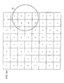
- FIGURE 6A through FIGURE 6E show steps that, by way of example, illustrate how cells are coalesced and split.
- Step 1 shows an initial division of the home region into a uniform grid.
- the area inside circle 61 has poor coverage, and the area outside has good coverage as shown by the number of "bad" counts in the respective cells.
- the cells with poor coverage have relatively large counts, and those with good coverage have relatively small counts.
- This initial arrangement has 64 cells, which, for illustration, we assume is all that the available memory will permit.
- the boundary of the region of poor coverage is marked by cells (or cell boundaries) with a small count on one side and a large count on the other.
- the system coalesces the grid elements whose incremented count densities are equal to their neighbors' count densities. Unless the service is very bad, most count densities will be equal (in the sense discussed above) to zero, so many cells will collapse into one, and the space required in the device memory for storage of data will be much less than for the original grid. Accordingly, memory is freed up if there is a large good area or a large bad area. As will be seen, this free memory is consumed by constructing an image of the boundary between good and bad areas. In principal, the boundary can be arbitrarily detailed, as long as it fits the available memory.
- Step 2 shows the effect after coalescing neighboring cells which have 'equal' count density.
- cells within 2 of one another are considered equal.
- the four center cells within circle 61 (circle 61 being a spatial boundary of the measured phenomenon, a portion of which is outside the home region of this measuring device) having counts of 20, 21, 20 and 19 (80) have been reduced to a single cell having a count of 80 which is the sum of the original cells.
- all the non-boundary cells (cells not on the boundary of the circle) to the left of circle 61 are reduced to a single cell having a count of 6.
- the three non-boundary cells (cells not on the boundary of the circle) above circle 61 are reduced to a single cell having a cell count of 3 while the nine non-boundary cells (cells not on the boundary of the circle) below circle 61 have been reduced to a single cell having a count of 1.
- Step 3 shows the result after splitting those cells which were not coalesced with their neighbors. There are now 36 cells based upon a 4 for 1 split of each coalesced cell. The boundary of the region of poor coverage is marked as in Step 1, but since those cells are now smaller, the boundary is determined more precisely.
- Step 4 shows the situation after the cells have been accumulating counts for some time. As would be expected, the cells in the area of poor coverage accumulate counts at a higher rate than do the cells in the better coverage areas.
- Step 5 shows the result after a second round of coalescing neighboring cells which have 'equal' count density, and then splitting the cells that remain. Note the three cells at the bottom of circle 61 which have not been split. There are 63 cells in this FIGURE; further splitting would require more memory than had been used (64) for the initial cell count (see step 1, FIGURE 6A). (In step 1, the assumption is that the available memory has all been used). The algorithm stops splitting when there is insufficient memory to do so. The boundary of the region of poor coverage is still marked as in Step 1, but since those cells are now smaller, the boundary is determined even more precisely.
- Places where the signal quality is different at different altitudes are treated the same as places where the signal quality is different at different times; i.e. there will probably not be a consistent hole. If mobile devices know their location in three dimensions than the concept discussed in this patent can be generalized to three dimensions. This would only be practical if sufficient memory exists. However, since mobile phone locating methods do not work very well indoors or underground, three dimensions may not be practical. Note that a device may have been in a "bad” location many times and for one reason or another (for example, being turned off) not logged a "bad" signal.
- FIGURE 7 shows RF system 700 having RF communication tower 701 controlled by control system 702.
- RF tower 701 is a cellular tower communicating to cell phones 50-1, 50-2 through 50-n. These cell phones are mobile and can thus move throughout the coverage area or to other areas. As they each move, they will each contain within the device the incremented numbers recorded according to the system and method discussed above. Periodically, this information will be communicated to control system 702 for the purpose of allowing the central system to then determine problems within the coverage areas based upon actually occurring criteria as determined from mobile devices in the course of their normal end-user usage. Note that the "home" region of each device is defined based upon that device's actual movements and thus each home region will be different. This difference then assures that the entire coverage area is monitored.
- the system and method described will over time compute the boundary of regions where the device was unable to support a call and will do this within fixed memory limits in a hand-held wireless device.
- the device will devote almost no memory to regions where service is adequate.
- the process will be more memory-efficient if there are a few large holes as opposed to many small ones.
- the devices used for example, the cellular phones, will be ones that are in the region naturally, because they are being used on a commercial network for which they were intended and not as a piece of extraneous test equipment.
- a cellular telephone is being used to make and receive calls and the population of cell phone users (not any particular one cell phone user) will tend to go into every possible location within any cellular region.
- the actual end-user device defines the locations for making measurements, and the region is not limited to places where test equipment can go. This then yields more natural test results since it is based on actual user experience over a wide population.
- This process evolves an ever-more-detailed image of the boundary of coverage holes, in bounded memory and using only 1-byte counters.
- the two main aspects of determining coverage locations and determining holes could run concurrently or alternately, or by constantly updating the counts in the cache, perhaps at a slower rate once the system has calculated a home location. Updating home location is necessary because the system might have made a wrong choice, or the user's behavior may have changed.
- the concepts taught herein can be used for detecting the boundary of any phenomenon, as long as it's fairly stationary and mobile devices can detect that phenomenon. For example, a determination can be made of where there's a lot of background noise; where traffic consistently speeds up or slows down; the level of smog (if smog sensors are placed on mobile devices) or sunlight (if correction is made for time of day), etc. Also, while a cellular system has been described, the concepts taught herein could be used for any type of communication or broadcast transmission system, including, by way of example, WIFI, Internet and wireless computing, radar, and sensor.
Landscapes
- Engineering & Computer Science (AREA)
- Computer Networks & Wireless Communication (AREA)
- Signal Processing (AREA)
- Mobile Radio Communication Systems (AREA)
Abstract
Description
- This disclosure relates to wireless coverage detection and more particularly to systems and methods for using mobile devices for detecting the boundary of a measurable phenomenon, such as the signal quality of RF broadcasts.
- Providers of wireless services, such as, for example, cellular telephone service, currently detect holes in their coverage in two ways, drive testing throughout the coverage area and customers calling to report problems. One disadvantage of drive testing is that the RF field is undersampled in time, since each sample covers only a fraction of a second per month at any one location. Another disadvantage of drive testing is that the RF field is also undersampled in space, because most of the major roads are not driven their entire length and only some of the minor roads are driven. Drive testing misses all locations without a road, such as parks, stadiums, homes, offices, conference centers, etc. While drive testing attempts to weigh the samples by their importance (making sure to cover major roads, for example) this weighing is subjective and ad hoc, and applies a single weighing for all customers. In addition, drive testing is labor-intensive and requires a truck full of expensive equipment. A disadvantage of having customers call in complaints is that such a system is subjective and undersamples the signal even more seriously than does drive testing, both in time and space. In addition, called-in information is usually imprecise and it is also labor-intensive to record the called-in data.
- In one embodiment there is shown a system and method for determining the spatial boundary of measurable phenomenon, such as the quality of a broadcast signal at various locations within geographical areas covered by the broadcast signal. Data representing relative signal quality at various locations within the geographical area is created within a mobile device, such as a cell phone capable of receiving the broadcast signals. The data is stored, and refined, within the device so as to define weak signal quality areas within at least a portion of the geographical area traveled by the mobile device. The data stored within the mobile device is from time to time communicated to the central broadcast system. The refinement of the data in the device allows for long storage periods so that signal quality can be reported over long time spans. By collecting such data from a plurality of such devices, the central system can map the signal strength over the entire geographical area.
- FIGURE 1A shows geographical areas defined by a mobile device;
- FIGURES 1B, 1C, and 1D show movement, expansion and contraction of the geographical area of FIGURE 1;
- FIGURES 2, 3, and 4 show flow charts of one embodiment of system operations;
- FIGURE 5 shows one embodiment of a mobile device;
- FIGURES 6A, 6B, 5C, 6D and 6E show one embodiment of the steps for changing the size of cells; and
- FIGURE 7 shows one embodiment of a cellular system using the systems and methods described herein.
- FIGURE 1A shows geographical area I 1 where the user of a mobile device (for example, a cellular telephone) spends most of his/her time. The letter 'A' is positioned at the center of
geographical area 11. For discussion purposes, this is called the 'home' region and in discussing FIGURES 1A-1D the method discussed with respect to FIGURE 2 will be used. - Assume now that the user moves a little bit and spends his/her time in
region 12 shown with a 'B' at its center. In thissituation region 11 will expand. FIGURE 1B shows the expandedregion 13. In FIGURE 1B the new home region has expanded on the north and east. - The expansion amount could be by just enough to include the user's new location or could be by an integral number of bins (cells), or by doubling the original size, etc.
- FIGURE 1C shows an example where the user remains within the confines of
region 12 and, periodically, as will be discussed hereinafter, the region is reduced. For discussion purposes herein it should be noted that acts performed periodically can be performed at regular intervals or at random intervals. In this example,region 12 is reduced on all sides to formregion 14. - FIGURE 1D shows that the home region, now
region 15, has again been expanded on the north and east to include areas of user movement. The home region now includes the new areas of user movement, and omits the areas where the user no longer goes. The home region has effectively moved to follow the user from A to B. - When the user goes far outside the home region (e.g., flies somewhere), the coordinates (and the data associated with the coordinates) are cached (home coordinate cache) and a new temporary region is created.
- In addition, the system periodically increments a count associated with the region the user is currently in and periodically deletes from the cache the region with the smallest count. When one region count exceeds some threshold, the system has established a home region. Using this method, the system establishes which cached region is the user's home region. There may be a tie, or a near-tie, for first place, depending on the usage pattern. However, this does not matter since the important thing is to choose a region where the user spends a lot of time. In the embodiment shown, it takes four numbers to store the bin information. The numbers may be, for example, latitude/longitude, or distance (in bins, or some other unit) plus an angle from a known tower, or some other coordinate system (which need not be Cartesian).
- By using more numbers: five (2 locations + angle) for a rotated rectangle, six for a triangle, eight for an arbitrary quadrilateral, etc. less restrictive region boundaries can be accommodated. To appreciate the value of less restrictive representations, imagine trying to represent a highway 100 feet wide and 20 miles long, running at a 45° angle. If the rectangle must have horizontal and vertical sides, it will be 14 miles on a side. If the system allows it to be rotated 45°, it only needs to be 100 feet on one side. The cache size of the home coordinate cache (as discussed above) can be as small as desired, as long as it contains at least two elements. The larger the cache, the greater the chance of converging quickly on "home."
- FIGURE 2 shows one embodiment of a flowchart showing system and
method 20 for determining the home region for storing data pertaining to signal strength.Process 201 starts with an initial home region. One embodiment for determining the home region is shown in FIGURE 3 to be discussed hereinafter. -
Process 202 determines whether the user has moved outside of the home region. If the user has moved outside the home region,process 203 determines if the user has moved beyond a given distance. If not, then the boundary is expanded viaprocess 204 as discussed above. If the user has moved beyond a given distance, then the prior region's data is stored in a cache viaprocess 205.Process 206 then determines if the new location is in cache. If so, that cached region becomes the new home region. If not, thenprocess 208 creates a new home region. -
Process 209 periodically increments the count for the current region andprocess 210 periodically shrinks the current region. Either or both of these actions can be incremented periodically, such as every minute (hour), (day), etc., as desired. While uniform shrinking is discussed, an important factor is that shrinkage (whether uniform or nonuniform) is unbiased over the long run. Thus, the shrinkage need not be uniform across the region, and one side could be reduced at one time and a different side reduced at another time. The side or sides to be reduced could be determined in order (north, south, east, west, etc.) or in random order, and any number of sides can be reduced at a time. - As discussed above, this system will continually refine itself so that if a user has moved to a new home region, the new home region will soon become the official home region and the system will continue without anything being done by either the user or the central system to which the device will eventually report. In addition, as discussed above, the size of the area will continually refine downward (or upward) so that as the user's movements reduce (or increase) the home region also reduces (or increases).
- FIGURE 3 shows one
embodiment 30 of a system and method for constructing a grid of cells describing the measurement of the phenomenon, for example, quality of wireless coverage.Process 301 constructs a cell grid over the region where the user presently is located. This cell grid can be as fine as memory will allow. Note that the memory can be different for different mobile devices, and thus, the size of grid area or the refinement therein can be different.Process 302 sets all cells to 0 initially.Processes 303 to 306 are several examples of a defined "bad" cell. In this context "bad" can be defined in any manner subjectively observable by the device and generally pertains to the quality of the signal. No signal is the ultimate bad quality. If desired, different levels of severity can cause a cell's count to be incremented more than once. Thus a dropped call is one example of a "bad" reading. If desired, bad readings can be graded such that a dropped call can be, say, the equivalent of two low RF signal readings, while other factors only give rise to a single incremented count. -
Process 303 determines if a call has been dropped. If so,process 313 determines the cell where the dropped call occurred and an incremented count is made in that cell viaprocess 323. As discussed, this increment would be, for example, a 1 added to the cell to show that a call has been dropped in that cell by this device. Again, note that this information is maintained in the device itself, and is not, at this point, communicated to the central system. -
Process 304 determines whether an attempted call has failed, if it has,process 314 finds which cell the call was attempted from. That cell is incremented viaprocess 324. - Process 305 to 305N checks for other failure modes and the proper cells are located and incremented via processes 315 to 315N and 325 to 325N.
-
Process 306 checks to see if a periodic check of strength has failed, and if so, then process 316 finds which cell the signal strength has failed in andprocess 326 increments that cell.Process 306 works under periodic control ofprocess 307 and can, if desired, be under random control, or triggered by external signals or any other manner desired. -
Process 308 determines whether a triggering event for reducing the region has occurred. If it has, then system andmethod 40, shown in FIGURE 4 is entered and, as will be discussed in more detail hereinafter, operates to reduce the memory required for the active region so that more data can be stored for faulty cells. -
Process 330, FIGURE 3, determines if it is time to file the data with the central system. If it is, then data, viaprocess 331, is transferred from the cell phone to the central system. This transfer can occur periodically, randomly, or on command from the central system as will be discussed, this time can be once a year, or every several months, or sooner as desired. At some point in time, it may be proper to reset the cells to 0. If so, then the system triggersprocess 302 and system andmethod 30 will repeat. - Note that for
processes - FIGURE 4 shows one
embodiment 40 of a system and method for refining the boundary of the region of poor coverage, by giving cells not on the boundary coarse granularity, and cells on the boundary fine granularity. Processes 401-402 control coarse granularity with respect to adjacent cells which have approximately equal density of counts per unit area. These approximately equal cells are merged into a single cell, and the cell's count is set equal to the sum of the counts of the merged cells. Note that this process frees up memory, which is used in later steps. There is, in general, more than one solution. For example, if there is an L-shaped region of equal density, a decision must be made with respect to the corner belonging to the vertical or the horizontal piece. Any choice can be made here, as long as the merged regions are rectangular. - Similarly, any reasonable interpretation of 'equal' will work - exactly equal, within "n" counts/area, within "n" percent, etc. Thus, a user can decide how to design the system and method to take into account the desired interpretation of "all cells are equal": (i.e.) the difference between neighbors is small, the difference between max and min is small, the difference between max and average is small, etc. Again, any method can be chosen, but it is good practice to use the difference between max and min; otherwise the method could be fooled by a smooth gradient.
- Processes 403-406 control fine granularity.
Process 403 divides each cell whose density is not "equal" to that of its neighbors into four cells. This uses the memory which was freed in the previous step. If there is not enough memory, as determined byprocess 404 to do this step, then division is ended as shown inprocess 403. -
Process 406 assigns a count to each new cell created inprocess 403. The count is chosen as follows. Assume the original cell's count is C. - (1) If C<4, then set p=C/4, and set each new cell's count to I with probability p, and 0 with probability 1-p.
- (2) If C is exactly divisible by 4, then set each new cell's count to C/4.
- (3) Otherwise, let R be the
remainder C mod 4, and let S=C-R. S is now exactly divisible by 4. Proceed as in step (1) with R and as in step (2) with S. - The above is but one embodiment for dividing the region near the boundary into smaller cells and partitioning the counts fairly. Any other method of representing the region as a hierarchic collection of variable-sized rectangles will also serve to keep the memory requirements approximately constant while providing detail near the boundary. For example, see Samet, H., 1988 "Hierarchical representation of collections of small rectangles." ACM Computing Surveys Vol. 20 No. 4, 271-309.
- FIGURE 5 shows one example of a hand-held
device 50. In the example,device 50 is a cellularphone having display 51,location detector 56, signalstrength detector 57,processor 53,memory 54 and counters 55. Some or all of these elements may not be necessary or can be combined into one or more as desired. Note that the mobile device can be any type of device designed to receive wireless broadcast signals, such as, for example cell phones, PDAs, navigation systems, computers, vehicle control processors, etc. - FIGURE 6A through FIGURE 6E show steps that, by way of example, illustrate how cells are coalesced and split.
-
Step 1, as shown in FIGURE 6A, shows an initial division of the home region into a uniform grid. The area insidecircle 61 has poor coverage, and the area outside has good coverage as shown by the number of "bad" counts in the respective cells. Thus, after some time has passed, the cells with poor coverage have relatively large counts, and those with good coverage have relatively small counts. This initial arrangement has 64 cells, which, for illustration, we assume is all that the available memory will permit. The boundary of the region of poor coverage is marked by cells (or cell boundaries) with a small count on one side and a large count on the other. - After some time, (which may be a timed interval, or when the largest count exceeds a threshold, or when the sum of counts exceeds a threshold), as shown by
process 308, FIGURE 3, the system coalesces the grid elements whose incremented count densities are equal to their neighbors' count densities. Unless the service is very bad, most count densities will be equal (in the sense discussed above) to zero, so many cells will collapse into one, and the space required in the device memory for storage of data will be much less than for the original grid. Accordingly, memory is freed up if there is a large good area or a large bad area. As will be seen, this free memory is consumed by constructing an image of the boundary between good and bad areas. In principal, the boundary can be arbitrarily detailed, as long as it fits the available memory. -
Step 2, as shown in FIGURE 6B, shows the effect after coalescing neighboring cells which have 'equal' count density. In this example, cells within 2 of one another are considered equal. There are now 12 cells. Note that the four center cells within circle 61 (circle 61 being a spatial boundary of the measured phenomenon, a portion of which is outside the home region of this measuring device) having counts of 20, 21, 20 and 19 (80) have been reduced to a single cell having a count of 80 which is the sum of the original cells. Also note that all the non-boundary cells (cells not on the boundary of the circle) to the left ofcircle 61 are reduced to a single cell having a count of 6. Likewise, the three non-boundary cells (cells not on the boundary of the circle) abovecircle 61 are reduced to a single cell having a cell count of 3 while the nine non-boundary cells (cells not on the boundary of the circle) belowcircle 61 have been reduced to a single cell having a count of 1. -
Step 3, as shown in FIGURE 6C, shows the result after splitting those cells which were not coalesced with their neighbors. There are now 36 cells based upon a 4 for 1 split of each coalesced cell. The boundary of the region of poor coverage is marked as inStep 1, but since those cells are now smaller, the boundary is determined more precisely. -
Step 4, as shown in FIGURE 6D, shows the situation after the cells have been accumulating counts for some time. As would be expected, the cells in the area of poor coverage accumulate counts at a higher rate than do the cells in the better coverage areas. -
Step 5, as shown in FIGURE 6E, shows the result after a second round of coalescing neighboring cells which have 'equal' count density, and then splitting the cells that remain. Note the three cells at the bottom ofcircle 61 which have not been split. There are 63 cells in this FIGURE; further splitting would require more memory than had been used (64) for the initial cell count (seestep 1, FIGURE 6A). (Instep 1, the assumption is that the available memory has all been used). The algorithm stops splitting when there is insufficient memory to do so. The boundary of the region of poor coverage is still marked as inStep 1, but since those cells are now smaller, the boundary is determined even more precisely. - This process continues, stopped only by running out of memory, or by being restarted by
process 332, FIGURE 3. Note that as shown in FIGURES 6A-6E the boundary of the measured "bad" (or out of norm) phenomenon need not lie entirely within the region reported by the device. Thus, it may take several devices to properly describe the totality of the "bad" phenomenon. - Places where the signal quality is different at different altitudes are treated the same as places where the signal quality is different at different times; i.e. there will probably not be a consistent hole. If mobile devices know their location in three dimensions than the concept discussed in this patent can be generalized to three dimensions. This would only be practical if sufficient memory exists. However, since mobile phone locating methods do not work very well indoors or underground, three dimensions may not be practical. Note that a device may have been in a "bad" location many times and for one reason or another (for example, being turned off) not logged a "bad" signal.
- FIGURE 7 shows
RF system 700 havingRF communication tower 701 controlled bycontrol system 702. In the embodiment shown,RF tower 701 is a cellular tower communicating to cell phones 50-1, 50-2 through 50-n. These cell phones are mobile and can thus move throughout the coverage area or to other areas. As they each move, they will each contain within the device the incremented numbers recorded according to the system and method discussed above. Periodically, this information will be communicated to controlsystem 702 for the purpose of allowing the central system to then determine problems within the coverage areas based upon actually occurring criteria as determined from mobile devices in the course of their normal end-user usage. Note that the "home" region of each device is defined based upon that device's actual movements and thus each home region will be different. This difference then assures that the entire coverage area is monitored. - The system and method described will over time compute the boundary of regions where the device was unable to support a call and will do this within fixed memory limits in a hand-held wireless device. The device will devote almost no memory to regions where service is adequate. The process will be more memory-efficient if there are a few large holes as opposed to many small ones. The devices used, for example, the cellular phones, will be ones that are in the region naturally, because they are being used on a commercial network for which they were intended and not as a piece of extraneous test equipment. Thus, in the embodiment shown, a cellular telephone is being used to make and receive calls and the population of cell phone users (not any particular one cell phone user) will tend to go into every possible location within any cellular region. Thus, the actual end-user device defines the locations for making measurements, and the region is not limited to places where test equipment can go. This then yields more natural test results since it is based on actual user experience over a wide population.
- A large portion of the device memory is spent storing counts of instances of poor service. The process is more accurate if it runs longer (assuming stationary service holes), but this requires larger counts, hence wider counters, hence more memory. If a user spends, say, 15 minutes a day in a coverage hole and the system samples every 10 seconds, then an 8-bit counter will overflow in 3 days. Morris, Robert "Counting Large Number Of Events In Small Registers" Communications of the ACM,
Volume 21 Number 10, pp. 841-842, October 1978, which is hereby incorporated by reference herein, developed a technique whereby the logarithm of the count can be stored (the technique does not require computing logarithms). The result is approximate, but since the system is sampling a continuous phenomenon, and "equal" is already approximate, it can accept an approximate count. Using the Morris method, and accepting a standard deviation of about 10%, an 8-bit counter's range can be extended to 4 years. One can use sub-byte counters, but this brings little benefit because the log function grows slowly. A 7-bit counter under these conditions will span just 3 weeks. This type of counter can also be used for the counts in the cache. - This process evolves an ever-more-detailed image of the boundary of coverage holes, in bounded memory and using only 1-byte counters. The two main aspects of determining coverage locations and determining holes could run concurrently or alternately, or by constantly updating the counts in the cache, perhaps at a slower rate once the system has calculated a home location. Updating home location is necessary because the system might have made a wrong choice, or the user's behavior may have changed.
- The concepts taught herein can be used for detecting the boundary of any phenomenon, as long as it's fairly stationary and mobile devices can detect that phenomenon. For example, a determination can be made of where there's a lot of background noise; where traffic consistently speeds up or slows down; the level of smog (if smog sensors are placed on mobile devices) or sunlight (if correction is made for time of day), etc. Also, while a cellular system has been described, the concepts taught herein could be used for any type of communication or broadcast transmission system, including, by way of example, WIFI, Internet and wireless computing, radar, and sensor.
- Although the present invention and its advantages have been described in detail, it should be understood that various changes, substitutions and alterations can be made herein without departing from the invention as defined by the appended claims. Moreover, the scope of the present application is not intended to be limited to the particular embodiments of the process, machine, manufacture, composition of matter, means, methods and steps described in the specification. As one will readily appreciate from the disclosure, processes, machines, manufacture, compositions of matter, means, methods, or steps, presently existing or later to be developed that perform substantially the same function or achieve substantially the same result as the corresponding embodiments described herein may be utilized. Accordingly, the appended claims are intended to include within their scope such processes, machines, manufacture, compositions of matter, means, methods, or steps.
Claims (10)
- A method for determining the spatial boundary of measurable phenomenon at various locations within geographical areas; said method comprising:measuring (30) relative quality of certain of said phenomenon at a defined region (20) within said geographical area, said measuring occurring within a mobile device (50) and resulting in measured data; said defined region being defined by the movement of said mobile device, andmaintaining within said device said measured data (323-326) so as to define poor quality areas within at least a portion of said defined region.
- The method of claim 1 further comprising:from time to time redefining said defined region (40) for each said mobile device.
- The method of claim 1 wherein said maintaining comprises:storing instances of poor quality cells (313-315) representing locations within said defined region; andfrom time to time (307) reassessing said cells.
- The method of claim 3 wherein said reassessing comprises coalescing (308) certain of said cells to form a single cell.
- The method of claim 3 wherein said reassessing comprises splitting certain cells to form several cells (403-406).
- The method of claim 3 wherein said coalescing comprises combining those cells whose count density of instances of poor quality are approximately equal (402).
- The method of claim 1 further comprising:communicating defined ones of said poor quality areas (330-331) from said device to a control system (700-702).
- A hand-held mobile device for receiving wireless signals; said device comprising:a poor signal quality indicator (57);a location detector (56); andmemory (54) for storing poor signal quality indications corresponding to a plurality of detected locations.
- The hand-held mobile device of claim 8 wherein said poor signal quality indication is an incremented count maintained within said device on a location by location basis (323-326), said locations being actual locations of each said device at the time said indication is incremented.
- The hand-held mobile device of claim 8 further comprising:a transmitter within said device (50) for sending from time to time said poor signal quality indications for at least one of said detected locations to a control point (700-702) external to said device.
Applications Claiming Priority (1)
| Application Number | Priority Date | Filing Date | Title |
|---|---|---|---|
| US10/909,814 US7356340B2 (en) | 2004-08-02 | 2004-08-02 | System and method for wireless coverage detection |
Publications (1)
| Publication Number | Publication Date |
|---|---|
| EP1626596A1 true EP1626596A1 (en) | 2006-02-15 |
Family
ID=35448028
Family Applications (1)
| Application Number | Title | Priority Date | Filing Date |
|---|---|---|---|
| EP05252866A Withdrawn EP1626596A1 (en) | 2004-08-02 | 2005-05-10 | System and method for wireless coverage detection |
Country Status (2)
| Country | Link |
|---|---|
| US (1) | US7356340B2 (en) |
| EP (1) | EP1626596A1 (en) |
Cited By (3)
| Publication number | Priority date | Publication date | Assignee | Title |
|---|---|---|---|---|
| WO2008045866A3 (en) * | 2006-10-12 | 2008-10-09 | Qualcomm Inc | Methods and apparatus for network re-creation in controlled environments |
| EP2096887A1 (en) * | 2008-02-29 | 2009-09-02 | Nokia Siemens Networks Oy | Apparatus and method for coverage hole detection, and uplink reporting |
| WO2009152097A1 (en) * | 2008-06-13 | 2009-12-17 | Qualcomm Incorporated | Apparatus and method for generating performance measurements in wireless networks |
Families Citing this family (16)
| Publication number | Priority date | Publication date | Assignee | Title |
|---|---|---|---|---|
| US7493103B2 (en) * | 2004-07-22 | 2009-02-17 | International Business Machines Corporation | Method and apparatus to transfer data and detect weak signals |
| US7236767B1 (en) * | 2005-06-03 | 2007-06-26 | Sprint Communications Company L.P. | Wireless cell site finder and customer service system |
| US8089407B2 (en) * | 2005-12-16 | 2012-01-03 | Alcatel Lucent | System and method for model-free position estimation and tracking |
| US8548502B2 (en) * | 2006-09-05 | 2013-10-01 | Broadcom Corporation | Spatial mapping of wireless access point service area |
| US20090040028A1 (en) * | 2007-05-31 | 2009-02-12 | Cms Products Inc | System and method for communicating data via a wireless high speed link between mobile computers and archival storage devices |
| WO2009003194A1 (en) * | 2007-06-27 | 2008-12-31 | T-Mobile Usa, Inc. | Method and system for a communications information interface |
| US8145186B1 (en) * | 2008-03-31 | 2012-03-27 | Sprint Communications Company L.P. | Assessing the comparative performance of telecommunication service areas |
| US8891442B2 (en) * | 2009-06-30 | 2014-11-18 | Clearwire Ip Holdings Llc | Apparatus and method for dual-mode operation |
| US8285291B2 (en) | 2010-02-02 | 2012-10-09 | Clearwire Ip Holdings Llc | System and method for multimode device handover |
| US8396039B2 (en) | 2010-04-15 | 2013-03-12 | Clearwire Ip Holdings Llc | Apparatus and method for multimode device handover |
| US8606260B2 (en) * | 2010-08-18 | 2013-12-10 | Apple Inc. | Location-based profile |
| CN103155662B (en) * | 2010-09-10 | 2017-04-05 | 诺基亚技术有限公司 | Set up signal intensity profile |
| US8666048B2 (en) * | 2012-04-18 | 2014-03-04 | International Business Machines Corporation | Location based quality of session control in unified telephony |
| CN108124279B (en) * | 2017-12-12 | 2021-06-08 | 中国联合网络通信集团有限公司 | Method and device for evaluating network coverage quality |
| CN110139209A (en) * | 2019-04-09 | 2019-08-16 | 武汉虹信技术服务有限责任公司 | A kind of vehicle module for 5G communication optimization |
| CN110611879B (en) * | 2019-09-11 | 2020-09-29 | 维沃移动通信有限公司 | Network parameter processing method, network side equipment and terminal |
Citations (4)
| Publication number | Priority date | Publication date | Assignee | Title |
|---|---|---|---|---|
| DE19533472A1 (en) * | 1995-09-12 | 1997-03-13 | Deutsche Telekom Mobil | Location of origin of measuring data for radio characteristics of cellular network |
| US6006089A (en) * | 1996-03-06 | 1999-12-21 | Leader Electronics Corp. | System and method of measuring electric field strength |
| US6266514B1 (en) * | 1998-11-06 | 2001-07-24 | Telefonaktiebolaget Lm Ericsson | Poor network coverage mapping |
| US20020042268A1 (en) * | 2000-08-15 | 2002-04-11 | Cotanis Nicolae G. | Systems and methods for determining signal coverage |
Family Cites Families (5)
| Publication number | Priority date | Publication date | Assignee | Title |
|---|---|---|---|---|
| AU726718B2 (en) * | 1996-11-18 | 2000-11-16 | Nokia Telecommunications Oy | Monitoring traffic in a mobile communication network |
| US6480718B1 (en) * | 1999-07-12 | 2002-11-12 | Nortel Networks Limited | Automatic frequency planning for a wireless network |
| US6708036B2 (en) * | 2001-06-19 | 2004-03-16 | Telcordia Technologies, Inc. | Methods and systems for adjusting sectors across coverage cells |
| US20030008619A1 (en) * | 2001-07-03 | 2003-01-09 | Werner Raymond J. | Location-based information service for identifying areas with degraded radio signal strength |
| US6799016B2 (en) * | 2001-09-21 | 2004-09-28 | Motorola, Inc. | Method for mapping poor coverage areas |
-
2004
- 2004-08-02 US US10/909,814 patent/US7356340B2/en not_active Expired - Fee Related
-
2005
- 2005-05-10 EP EP05252866A patent/EP1626596A1/en not_active Withdrawn
Patent Citations (4)
| Publication number | Priority date | Publication date | Assignee | Title |
|---|---|---|---|---|
| DE19533472A1 (en) * | 1995-09-12 | 1997-03-13 | Deutsche Telekom Mobil | Location of origin of measuring data for radio characteristics of cellular network |
| US6006089A (en) * | 1996-03-06 | 1999-12-21 | Leader Electronics Corp. | System and method of measuring electric field strength |
| US6266514B1 (en) * | 1998-11-06 | 2001-07-24 | Telefonaktiebolaget Lm Ericsson | Poor network coverage mapping |
| US20020042268A1 (en) * | 2000-08-15 | 2002-04-11 | Cotanis Nicolae G. | Systems and methods for determining signal coverage |
Cited By (7)
| Publication number | Priority date | Publication date | Assignee | Title |
|---|---|---|---|---|
| WO2008045866A3 (en) * | 2006-10-12 | 2008-10-09 | Qualcomm Inc | Methods and apparatus for network re-creation in controlled environments |
| US7840382B2 (en) | 2006-10-12 | 2010-11-23 | Qualcomm Incorporated | Methods and apparatus for network re-creation in controlled environments |
| EP2096887A1 (en) * | 2008-02-29 | 2009-09-02 | Nokia Siemens Networks Oy | Apparatus and method for coverage hole detection, and uplink reporting |
| WO2009152097A1 (en) * | 2008-06-13 | 2009-12-17 | Qualcomm Incorporated | Apparatus and method for generating performance measurements in wireless networks |
| US8098590B2 (en) | 2008-06-13 | 2012-01-17 | Qualcomm Incorporated | Apparatus and method for generating performance measurements in wireless networks |
| KR101213203B1 (en) | 2008-06-13 | 2012-12-18 | 콸콤 인코포레이티드 | Apparatus and method for generating performance measurements in wireless netowrks |
| RU2482621C2 (en) * | 2008-06-13 | 2013-05-20 | Квэлкомм Инкорпорейтед | Apparatus and method of generating measurements of technical characteristics in wireless networks |
Also Published As
| Publication number | Publication date |
|---|---|
| US7356340B2 (en) | 2008-04-08 |
| US20060025142A1 (en) | 2006-02-02 |
Similar Documents
| Publication | Publication Date | Title |
|---|---|---|
| US7356340B2 (en) | System and method for wireless coverage detection | |
| US7120449B1 (en) | Location determination in telecommunication network | |
| US20100103868A1 (en) | Method for modeling wireless network coverage under line-of-sight conditions | |
| AU674384B2 (en) | A mobile phone testing arrangement | |
| CN112506972B (en) | User resident area positioning method and device, electronic equipment and storage medium | |
| Zagatti et al. | A trip to work: Estimation of origin and destination of commuting patterns in the main metropolitan regions of Haiti using CDR | |
| US9220016B2 (en) | Position monitoring for a coverage area | |
| CN1148095C (en) | Mobile telephone system | |
| CN101426206A (en) | Method and system for gridding communication network call distribution | |
| CN106550386B (en) | A kind of detection method and device of antenna-feeder system | |
| CN114885287B (en) | Network coverage area determining method and device, electronic equipment and storage medium | |
| KR20060090303A (en) | Method and apparatus for determining gap in mobile phone area coverage | |
| US8010101B2 (en) | System and method for diagnosing RF attributes over an RF footprint of a wireless network | |
| CN106528675A (en) | Complaint reason positioning method and device | |
| CN113645625B (en) | Pseudo base station positioning method, pseudo base station positioning device, electronic equipment and readable medium | |
| CN113873431B (en) | Building network quality presentation method and device | |
| WO2009093239A2 (en) | A method for detecting events on cellular comm. network | |
| US6041239A (en) | Method and apparatus for distributing offered load in a wireless communications system | |
| US20200187148A1 (en) | Method of considering the positions of data points in relation to boundaries represented in a geographic information system database, in estimating location | |
| US20060094438A1 (en) | System and method for determining user-perceived holes in wireless communication coverage areas | |
| CN113133049B (en) | Method, apparatus, device and medium for determining primary coverage cell | |
| CN118139166A (en) | Resident position identification method based on space-time big data | |
| CN109257756A (en) | Indoor wireless networks method for evaluating quality and server | |
| CN113573236A (en) | Method and device for evaluating confidence of positioning result | |
| TWI418836B (en) | Wireless network signal collection and verification system |
Legal Events
| Date | Code | Title | Description |
|---|---|---|---|
| PUAI | Public reference made under article 153(3) epc to a published international application that has entered the european phase |
Free format text: ORIGINAL CODE: 0009012 |
|
| AK | Designated contracting states |
Kind code of ref document: A1 Designated state(s): AT BE BG CH CY CZ DE DK EE ES FI FR GB GR HU IE IS IT LI LT LU MC NL PL PT RO SE SI SK TR |
|
| AX | Request for extension of the european patent |
Extension state: AL BA HR LV MK YU |
|
| 17P | Request for examination filed |
Effective date: 20060814 |
|
| AKX | Designation fees paid |
Designated state(s): DE FR GB |
|
| 17Q | First examination report despatched |
Effective date: 20061011 |
|
| RAP1 | Party data changed (applicant data changed or rights of an application transferred) |
Owner name: AGILENT TECHNOLOGIES, INC. |
|
| STAA | Information on the status of an ep patent application or granted ep patent |
Free format text: STATUS: THE APPLICATION IS DEEMED TO BE WITHDRAWN |
|
| 18D | Application deemed to be withdrawn |
Effective date: 20081202 |