EP1473574A1 - Method of optimizing NMR measurement condition - Google Patents
Method of optimizing NMR measurement condition Download PDFInfo
- Publication number
- EP1473574A1 EP1473574A1 EP04251593A EP04251593A EP1473574A1 EP 1473574 A1 EP1473574 A1 EP 1473574A1 EP 04251593 A EP04251593 A EP 04251593A EP 04251593 A EP04251593 A EP 04251593A EP 1473574 A1 EP1473574 A1 EP 1473574A1
- Authority
- EP
- European Patent Office
- Prior art keywords
- pulse width
- mabn
- measurement condition
- value
- results
- Prior art date
- Legal status (The legal status is an assumption and is not a legal conclusion. Google has not performed a legal analysis and makes no representation as to the accuracy of the status listed.)
- Granted
Links
- 238000000034 method Methods 0.000 title claims abstract description 95
- 238000005481 NMR spectroscopy Methods 0.000 title claims abstract description 56
- 238000005259 measurement Methods 0.000 claims abstract description 112
- 238000001208 nuclear magnetic resonance pulse sequence Methods 0.000 claims description 29
- 238000005570 heteronuclear single quantum coherence Methods 0.000 claims description 7
- 238000012887 quadratic function Methods 0.000 claims 3
- 239000000523 sample Substances 0.000 description 22
- 238000010586 diagram Methods 0.000 description 15
- 238000012545 processing Methods 0.000 description 15
- 230000000007 visual effect Effects 0.000 description 13
- 238000000238 one-dimensional nuclear magnetic resonance spectroscopy Methods 0.000 description 10
- 229910001868 water Inorganic materials 0.000 description 9
- XLYOFNOQVPJJNP-UHFFFAOYSA-N water Substances O XLYOFNOQVPJJNP-UHFFFAOYSA-N 0.000 description 6
- 238000011156 evaluation Methods 0.000 description 5
- 238000009825 accumulation Methods 0.000 description 4
- 230000035508 accumulation Effects 0.000 description 4
- OKKJLVBELUTLKV-UHFFFAOYSA-N Methanol Chemical compound OC OKKJLVBELUTLKV-UHFFFAOYSA-N 0.000 description 3
- 238000003491 array Methods 0.000 description 3
- 238000005457 optimization Methods 0.000 description 3
- 230000003068 static effect Effects 0.000 description 3
- IAZDPXIOMUYVGZ-WFGJKAKNSA-N Dimethyl sulfoxide Chemical compound [2H]C([2H])([2H])S(=O)C([2H])([2H])[2H] IAZDPXIOMUYVGZ-WFGJKAKNSA-N 0.000 description 2
- 238000007429 general method Methods 0.000 description 2
- 230000001678 irradiating effect Effects 0.000 description 2
- 239000000126 substance Substances 0.000 description 2
- 239000004956 Amodel Substances 0.000 description 1
- 102000016943 Muramidase Human genes 0.000 description 1
- 108010014251 Muramidase Proteins 0.000 description 1
- 108010062010 N-Acetylmuramoyl-L-alanine Amidase Proteins 0.000 description 1
- 102000044159 Ubiquitin Human genes 0.000 description 1
- 108090000848 Ubiquitin Proteins 0.000 description 1
- XSQUKJJJFZCRTK-UHFFFAOYSA-N Urea Chemical compound NC(N)=O XSQUKJJJFZCRTK-UHFFFAOYSA-N 0.000 description 1
- 238000013459 approach Methods 0.000 description 1
- 239000004202 carbamide Substances 0.000 description 1
- ORTQZVOHEJQUHG-UHFFFAOYSA-L copper(II) chloride Chemical compound Cl[Cu]Cl ORTQZVOHEJQUHG-UHFFFAOYSA-L 0.000 description 1
- 229960003280 cupric chloride Drugs 0.000 description 1
- 230000007423 decrease Effects 0.000 description 1
- 238000012594 liquid chromatography nuclear magnetic resonance Methods 0.000 description 1
- 229960000274 lysozyme Drugs 0.000 description 1
- 235000010335 lysozyme Nutrition 0.000 description 1
- 239000004325 lysozyme Substances 0.000 description 1
- 238000000655 nuclear magnetic resonance spectrum Methods 0.000 description 1
- 238000005070 sampling Methods 0.000 description 1
- 230000003595 spectral effect Effects 0.000 description 1
Images


















Classifications
-
- G—PHYSICS
- G01—MEASURING; TESTING
- G01R—MEASURING ELECTRIC VARIABLES; MEASURING MAGNETIC VARIABLES
- G01R33/00—Arrangements or instruments for measuring magnetic variables
- G01R33/20—Arrangements or instruments for measuring magnetic variables involving magnetic resonance
- G01R33/44—Arrangements or instruments for measuring magnetic variables involving magnetic resonance using nuclear magnetic resonance [NMR]
- G01R33/48—NMR imaging systems
- G01R33/58—Calibration of imaging systems, e.g. using test probes, Phantoms; Calibration objects or fiducial markers such as active or passive RF coils surrounding an MR active material
- G01R33/583—Calibration of signal excitation or detection systems, e.g. for optimal RF excitation power or frequency
-
- G—PHYSICS
- G01—MEASURING; TESTING
- G01R—MEASURING ELECTRIC VARIABLES; MEASURING MAGNETIC VARIABLES
- G01R33/00—Arrangements or instruments for measuring magnetic variables
- G01R33/20—Arrangements or instruments for measuring magnetic variables involving magnetic resonance
- G01R33/44—Arrangements or instruments for measuring magnetic variables involving magnetic resonance using nuclear magnetic resonance [NMR]
- G01R33/46—NMR spectroscopy
-
- G—PHYSICS
- G01—MEASURING; TESTING
- G01R—MEASURING ELECTRIC VARIABLES; MEASURING MAGNETIC VARIABLES
- G01R33/00—Arrangements or instruments for measuring magnetic variables
- G01R33/20—Arrangements or instruments for measuring magnetic variables involving magnetic resonance
- G01R33/44—Arrangements or instruments for measuring magnetic variables involving magnetic resonance using nuclear magnetic resonance [NMR]
- G01R33/48—NMR imaging systems
- G01R33/54—Signal processing systems, e.g. using pulse sequences ; Generation or control of pulse sequences; Operator console
Definitions
- the present invention relates to a method of optimizing a measurement condition in an NMR measurement.
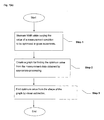
- Fig. 1 illustrates the prior art method of optimizing an NMR measurement condition.
- Fig. 1 (a) is a flowchart illustrating a general procedure for finding an optimum value of a measurement condition.
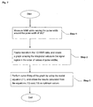
- Fig. 1 (b) is a flowchart illustrating a procedure for finding optimum values of RF pulse widths.
- Fig. 1(c) is a diagram illustrating a pulse sequence for measurement of an RF pulse width.
- step 1 NMR measurements are carried out while varying the value of a measurement condition to be optimized in given increments.
- step 2 a graph for finding the optimum value from the obtained measurement data by appropriate processing is created. At this time, varying value of the measurement condition is plotted on one axis of the graph.
- step 3 the optimum value is found from the shape of the graph by visual estimation.
- step 1 NMR measurements are performed while varying the pulse width from 0 to 70 ⁇ s using a pulse sequence shown in Fig. 1 (c) , for example, under measurement conditions listed in Table 1.
- Measurement condition set 1 under which measurements are performed with varying RF pulse width
- Item Value Sample 15 mM copper dichloride/1 % H 2 O, 99%D 2 O Magnetic field intensity 14.09636928 T Observed nucleus 1 H Observe frequency 600.1723046 MHz Center frequency of observation about 4.7 ppm (resonance frequency of water) Number of data points 16384 Sweep width 9.00252071 kHz Number of accumulations 1 B 1 pulse intensity about 25 kHz Observation time 1.81993472 s Relaxation_ delay 1 s Temperature 25°C
- [relaxation_delay] indicates the wait time of each repetition pulse. In this example, the time is 1 s.
- [x_pulse] indicates an RF pulse.
- NMR measurements are performed using a pulse width varied from 0 to 70 ⁇ s.
- [acquisition] indicates an observation.
- the time necessary for an observation is 1.81993472 s as shown in Table 1.
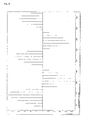
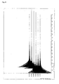
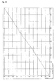
- Fig. 2 Data obtained from a measurement is shown in Fig. 2, where one-dimensional (1D) NMR data obtained using a certain pulse width are arrayed in the order of values of pulse widths at intervals of 2 ⁇ s.
- step 2 the obtained NMR data are first Fourier-transformed.
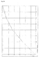
- the resulting data are shown in Fig. 3, where the data are arrayed in the order of values of pulse widths at intervals of 2 ⁇ s in the same way as in Fig. 2.
- a range from 4 to 5.5 ppm in the signal region is displayed.
- the data are arrayed horizontally in the order of values of pulse widths.
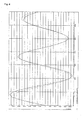
- the obtained graph is shown in Fig. 4, where the horizontal axis indicates the pulse width, while the vertical axis indicates the intensity of the NMR spectrum.
- step 3 a waveform formed by connecting the vertices of spectral intensities of Fig. 4 by means of straight lines is regarded as a sinusoidal (SIN) wave.
- SIN sinusoidal
- Patent Reference 1 Japanese Patent Laid-Open No. H3-139330.
- NMR scans are made with RF exciting field intensities of different arrays.
- a curve is applied to each set of corresponding data elements in one set of intensity arrays.
- the peaks of the applied curves are determined.
- Corresponding data in the transmit and receive arrays are generated from the determined peaks.
- a magnetic field map indicating nonuniformities in an RF magnetic field by means of the magnitudes of data elements is created.
- the prior art method of finding the optimum RF pulse width has the problem that the reliability of the optimum value is low, because the value is found from a created graph by visual estimation.
- it is necessary to increase the number of measurement data items. This prolongs the measurement time. If the number of measurement data items is reduced to shorten the measurement time, the reliability of the obtained optimum value deteriorates.
- Patent Reference 1 does not disclose a technique for optimizing measurement conditions, though the reference discloses a technique quantitatively indicating nonuniformities in transmit and receive fields.
- the present invention is intended to address the foregoing problems. It would be desirable to provide a technique for finding a reliable optimum value of a measurement condition with a reduced number of measurement data items, i.e., in a short time.
- a method of optimizing an NMR measurement condition in accordance with the invention starts with gaining NMR measurement data while varying the value of the measurement condition to be optimized. Then, a certain property is extracted as a numerical value from the measurement data. A plot is made along the varied value of the measurement condition to create a curve. Amodel equation coincident with the measurement condition, its range, and the certain property extracted as a numerical value is established. Curve fitting in which constants of the model equation are varied is done such that the equation agrees with the created curve. Constant values of the model equation and their standard deviation are obtained by curve fitting. An optimum value of the measurement condition is obtained from the results.
- curve fitting is used and so a good result can be obtained if the number of data items is reduced as long as they characterize a waveform.
- a reliable optimum value of a measurement condition can be found in a short time.
- Embodiments 1-5 pertain to a method of finding an optimum value of an RF pulse width using integrated values in the signal region.
- Embodiments 6-10 pertain to a method of finding an optimum value of an RF pulse width using peak top intensities of a signal.
- the measurement conditions of Table 1 and the pulse sequence of Fig. 1(c) are used.
- the invention is not restricted to the measurement conditions of Table 1 and pulse sequence of Fig. 1 (c) .
- Embodiment 11 pertains to a general method of optimizing an NMR measurement condition.
- the unit name "abn" in the various tables is identical with the unit name "au” and means a unitless intensity or magnitude.
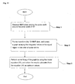
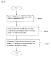
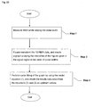
- Fig. 5 is a flowchart illustrating Embodiment 1 of the invention.
- (a) of Fig. 5 illustrates a procedure for finding an optimum value of an RF pulse width.
- (b) of Fig. 5 illustrates a procedure for finding an initial value in a DFP method (described later) .
- Embodiment 1 is a method of finding an optimum RF pulse width by measuring the pulse width over the whole range.
- step 1 NMR measurements are performed while varying an RF pulse width from 0 to 70 ⁇ s in increments of 2 ⁇ s, using the measurement conditions shown in Table 1 and pulse sequence shown in Fig. 1 (c) , for example. As a result, measurement data shown in Fig. 2 are obtained.
- step 2 the measurement data are Fourier-transformed, and a plot is done along the values of the RF pulse width using integrated values in the signal region. In this way, a curve is created.
- This processing results in data as shown in Fig. 3. Finding the integrated values from a signal range from 4 to 5.5 ppm produces results listed in Table 2. Plotting the results gives rise to the curve indicated by the solid line in Fig. 6.
- step 3 curve fitting (described later) is performed in which the constants A, B, C, D, and ⁇ of model equation (1) (given later) are varied such that model equation (1) agrees with the curve indicated by the solid line in Fig. 6.
- Model equation (1) (Eq. (1)), Eq. (2) for finding a 360° RF pulse width, and Eq. (3) for finding a 90° RF pulse width are given below.
- Curve fitting is to find the A, B, C, D, and ⁇ which minimize the following evaluation formula (4) using a multi-dimensional variable metric method (Davidon-Fletcher-Powell (DFP) method) described herein as Reference 1 (Numerical Recipes in C: THE ART OF SCIENTIFIC COMPUTING, Second Edition (ISEN 0-521-43108-5), 1992, pp. 425-430) .
- DFP Davidon-Fletcher-Powell
- the DFP method needs an evaluation equation and initial values.
- Eq. (4) using Eq. (5) identical with Eq. (1) is employed as this evaluation formula.
- t is an RF pulse width
- PWstart is the start value of the RF pulse width
- PWend is the end value of the width
- g(t) is the actually measured value of the intensity at the RF pulse width of t.
- the theoretical value f(t) of intensity is defined by Eq. (5) and equal to the right side of Eq. (1).
- LPSVD Linear Prediction Singular Value Deconvolution
- step 2 if calculations using the LPSVD method are unsuccessful, the program goes to step 3. If the calculations are successful, the program goes to step 7.
- the results are shown in Table 4.
- Intersection 1 with y 0 Item Value n 1 5 zp[1] 0.00016 ⁇ s zp[2] 15.44153 ⁇ s zp[3] 29.20118 ⁇ s zp[4] 43.63471 ⁇ s zp[5] 57.48084 ⁇ s
- step 4 the results shown in Table 4 are substituted into Eq. (6).
- ⁇ 0.21862 rad/ ⁇ s.
- ⁇ ⁇ ⁇ ( n 1 - 1) zp [ n 1 ]- zp [1]
- step 5 the number of positive-going (upward) peaks n 2 of the curve indicated by the solid line in Fig. 6, the RF pulse widths pp[1], .., pp[n 2 ] at the tops of the peaks, and the intensities pi [1] , ..., pi[n 2 ] of the tops of the peaks are found.
- the results are listed in Table 5.
- Tops 1 of peaks Item Value n 2 3 pp[1] 8 ⁇ s pp[2] 36 ⁇ s pp[3] 64 ⁇ s pi[1] 134.78419 kabn pi[2] 105.83569 kabn pi[3] 85.13906 kabn
- step 6 the results shown in Table 5 are substituted into Eq. (7).
- We obtain 121.90106 ⁇ s as an initial value of C ( C 121.90106 ⁇ s).
- step 7 the values of ⁇ and C calculated in step 1 or steps 4 and 6 are substituted into Eq. (8) that is an expansion of Eq. (5).
- Eq. (8) an expansion of Eq. (5).
- Table 6 uses the results of step 1.
- A E 2 + F 2 Results 1 of calculations of linear least squares method Item Value D 5381.95203 kabn E 119968.83441 kabn F -6577.86175999999 kabn
- the step of obtaining an optimum RF pulse width contains no manual operation and so reproducible results can be obtained.
- the number of data items is set equal to the number of data items used in the prior art procedure for convenience of illustration.
- curve fitting in a case where there are data points characterizing a waveform, if the number of data points is reduced, similar results can be obtained. Therefore, good results can be obtained if there are a reduced number of data items. This similarly applies to embodiments described later.
- Embodiment 2 of the invention is described next with reference to Fig. 7.
- Embodiment 2 is a method of finding an optimum RF pulse width by performing NMR measurements while varying the pulse width in the neighborhood of 360° pulse width.
- the 360° pulse width is 28 ⁇ s because of the technique described as the prior art or information obtained from other technique.
- step 1 NMR measurements are performed while varying an RF pulse width from 24 to 34 ⁇ s (i.e., around 360° pulse width) in increments of 2 ⁇ s, using the measurement conditions shown in Table 1 and pulse sequence shown in Fig. 1 (c) , for example. Measurement data shown in Fig. 8 are obtained.
- step 2 the measurement data are Fourier-transformed, and integrated values in the signal region are plotted along the values of the RF pulse width. In this way, a curve is created.
- the step of obtaining the RF pulse width does not use visual estimation. Therefore, reproducible results can be obtained.
- Embodiment 3 of the invention is next described with reference to Fig. 11.
- Embodiment 3 is a method of finding an optimum RF pulse width by performing NMR measurements while varying the pulse width in the neighborhood of 90° pulse width.
- the 90° pulse width is 7 ⁇ s because of the technique described as the prior art or information obtained from other technique.
- step 1 NMR measurements are performed while varying an RF pulse width from 4 to 12 ⁇ s (i.e., around 90° pulse width) in increments of 2 ⁇ s, using the measurement conditions shown in Table 1 and pulse sequence shown in Fig. 1(c), for example. Measurement data shown in Fig. 12 are obtained.
- step 2 the measurement data are Fourier-transformed, and integrated values in the signal region are plotted along the values of the RF pulse width. In this way, a curve is created.
- This processing results in data shown in Fig. 13.
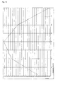
- Finding the integrated values from a signal existing region from 4 to 5.5 ppm produces results listed in Table 9. Plotting the results gives rise to the curve indicated by the solid line in Fig. 14.
- the step of obtaining the RF pulse width does not use visual estimation. Therefore, reproducible results can be obtained.
- Embodiment 4 of the invention is next described with reference to Fig. 15.
- Embodiment 4 is a method of finding an optimum RF pulse width by performing NMR measurements while varying the pulse width in the neighborhood of 180° pulse width.
- the 180° pulse width is 14 ⁇ s because of the technique described as the prior art or information obtained from other technique.
- step 1 NMR measurements are performed while varying an RF pulse width from 12 to 18 ⁇ s (i.e., around 180° pulse width) in increments of 2 ⁇ s, using the measurement conditions shown in Table 1 and pulse sequence shown in Fig. 1 (c) , for example. Measurement data shown in Fig. 16 are obtained.
- step 2 the measurement data are Fourier-transformed, and integrated values in the signal region are plotted along the values of the RF pulse width. In this way, a curve is created.
- This processing results in data shown in Fig. 17.
- Finding the integrated values from a signal existing range from 4 to 5.5 ppm produces results listed in Table 11. Plotting the results gives rise to the curve indicated by the solid line in Fig. 18.
- step 3 the linear least squares method is implemented using model equation (11). Results shown in Table 12 are obtained. Plotting of the contents of Table 12 using model equation (11) results in the curve indicated by the broken line in Fig. 19. Results 4 of calculations of curve fitting Constant Value A -12.32673 Mabn/ ⁇ s B 190.83045 Mabn ⁇ 0.66926 Mabn
- Embodiment 5 of the invention is next described by referring to Fig. 19.
- Embodiment 5 is a method of finding an optimum RF pulse width by performing NMR measurements while varying the pulse width in the neighborhood of 270° pulse width.
- the 270° pulse width is 21 ⁇ s because of the technique described as the prior art or information obtained from other technique.
- step 1 NMR measurements are performed while varying an RF pulse width from 18 to 26 ⁇ s (i.e., around 270° pulse width) in increments of 2 ⁇ s, using the measurement conditions shown in Table 1 and pulse sequence shown in Fig. 1 (c) , for example. Measurement data shown in Fig. 20 are obtained.
- step 2 the measurement data are Fourier-transformed, and integrated values in the signal region are plotted along the values of the RF pulse width. In this way, a curve is created.
- This processing results in data shown in Fig. 21.
- Finding the integrated values from a signal existing region from 4 to 5.5 ppm produces results listed in Table 13. Plotting the results gives rise to the curve indicated by the solid line in Fig. 22.
- step 3 the linear least squares method is implemented using model equation (13). Results shown in Table 14 are obtained. Plotting of the contents of Table 14 using model equation (13) results in the curve indicated by the broken line in Fig. 22. Results 5 of calculations of curve fitting Constant Value A 1.27911 Mabn/ ⁇ s 2 B -56.83557 Mabn/ ⁇ s C 577.97661 Mabn ⁇ 0.12472 Mabn
- the step of obtaining the RF pulse width does not use visual estimation. Therefore, reproducible results can be obtained.
- Embodiment 6 of the invention is described with reference to Fig. 23.
- Embodiment 6 is a method of finding an optimum RF pulse width by performing NMR measurements while varying the pulse width in a range from 0 to 360° and using peak top intensities of a signal.
- step 1 NMR measurements are performed while varying an RF pulse width from 0 to 70 ⁇ s in increments of 2 ⁇ s, using the measurement conditions shown in Table 1 and pulse sequence shown in Fig. 1(c), for example. Measurement data shown in Fig. 2 are obtained.
- step 2 the measurement data are Fourier-transformed, and the top intensities of maximum peaks in the signal region are plotted along the values of the RF pulse width.
- This processing results in data as shown in Fig. 3. Finding the maximum peak top intensities in the signal existing region from 4 to 5.5 ppm produces results listed in Table 15. Plotting the results gives rise to the curve indicated by the solid line in Fig. 24.
- step 3 a curve fitting DFP method is performed in which the constants A, B, C, D, and ⁇ of model equation (1) are varied such that model equation (1) agrees with the curve. Consequently, results shown in Table 16 are obtained. Results 6 of calculations of curve fitting Constant Value A 5780247.97088 abn B 0 rad C 165.63334 ⁇ s D 12119.0114 abn ⁇ 0.21641 rad/ ⁇ s ⁇ 964882.75674 abn
- step 1 the LPSVD method is used but calculations are unsuccessfully performed with no results.
- step 4 the results shown in Table 17 are substituted into Eq. (6).
- ⁇ 0.21846 rad/ ⁇ s.
- step 5 the number of positive-going (upward) peaks n 2 of the curve indicated by the solid line of Fig. 24, the RF pulse widths pp [1] , .., pp [n 2 ] at the tops of the peaks, and the intensities pi [1] , ..., pi [n 2 ] of the tops of the peaks are found. Results listed in Table 18 are obtained. Tops 2 of peaks Item Value n 2 3 pp[1] 10 ⁇ s pp[2] 38 ⁇ s pp[3] 66 ⁇ s pi[1] 5.79026 Mabn pi[2] 4.73415 Mabn pi[3] 3.94934 Mabn
- step 6 the results shown in Table 18 are substituted into Eq. (7).
- C 146.35619 ⁇ s as an initial value of C .
- step 7 the values of ⁇ and C calculated in steps 4 and 6 are substituted into Eq. (8).
- the linear least squares method is implemented. Results (optimum constant values D, E, and F ) listed in Table 19 are obtained. Results 2 of calculations of linear least squares method Item Value D 46209.1885 abn E 5919590.1939 abn F -796281.22262 abn
- the values calculated in this way are taken as initial values in the DFP method. These values are varied.
- the values of A, B, C, D, and ⁇ that minimize the value of evaluation formula (4) are found.
- the step of obtaining an optimum RF pulse width contains no manual operation and so reproducible results can be obtained.
- Embodiment 7 of the invention is described by referring to Fig. 25.
- Embodiment 7 is a method of finding an optimum RF pulse width by performing NMR measurements while varying the RF pulse width in the neighborhood of 360° pulse width.
- the 360° pulse width is 28 ⁇ s because of the technique described as the prior art or information obtained from other technique.
- step 1 NMR measurements are performed while varying an RF pulse width from 24 to 34 ⁇ s (i.e., around 360° pulse width) in increments of 2 ⁇ s, using the measurement conditions shown in Table 1 and pulse sequence shown in Fig. 1(c), for example. Measurement data shown in Fig. 8 are obtained.
- step 2 the measurement data are Fourier-transformed, and the top intensities of maximum peaks in the signal region are plotted along the values of the RF pulse width.
- This processing results in data as shown in Fig. 9. Finding the top intensities of maximum peaks in a signal existing region from 4 to 5.5 ppm produces results listed in Table 20. Plotting the results gives rise to the curve indicated by the solid line in Fig. 26.
- step 3 the linear least squares method is implemented using model equation (11). Results shown in Table 21 are obtained. Plotting of the contents of Table 21 using model equation (11) results in the curve indicated by the broken line in Fig. 26. Results 7 of calculations of curve fitting Constant Value A 1.1022 Mabn/ ⁇ s B -32.41038 Mabn ⁇ 0.11171 Mabn
- the step of obtaining an optimum RF pulse width does not use visual estimation. Therefore, reproducible results can be obtained.
- Embodiment 8 of the invention is next described with reference to Fig. 27.
- Embodiment 8 is a method of finding an optimum RF pulse width by performing NMR measurements while varying the RF pulse width in the neighborhood of 90° pulse width and by using the peak top intensities of the signal.
- the 90° pulse width is 7 ⁇ s because of the technique described as the prior art or information obtained from other technique.
- step 1 NMR measurements are performed while varying an RF pulse width from 4 to 12 ⁇ s (i.e., around 90° pulse width) in increments of 2 ⁇ s, using the measurement conditions shown in Table 1 and pulse sequence shown in Fig. 1(c). Measurement data shown in Fig. 12 are obtained.
- step 2 the measurement data are Fourier-transformed, and the top intensities of the maximum peaks in the signal region are plotted along the values of the RF pulse width.
- This processing results in data shown in Fig. 13.
- Finding the top intensities of the maximum peaks in a signal existing range from 4 to 5.5 ppm produces results listed in Table 22. Plotting the results gives rise to the curve indicated by the solid line in Fig. 28.
- step 3 the linear least squares method is implemented using model equation (13). Results shown in Table 23 are obtained. Plotting of the contents of Table 23 using model equation (13) results in the curve indicated by the broken line in Fig. 28. Results 8 of calculations of curve fitting Constant Value A -0.069719 Mabn/ ⁇ s 2 B 1.83886 Mabn/ ⁇ s C -1.99495 Mabn ⁇ 0.06976 Mabn
- the step of obtaining the optimum RFpulse width does not use visual estimation. Therefore, reproducible results can be obtained.
- Embodiment 9 of the invention is described by referring to Fig. 29.
- Embodiment 9 is a method of finding an optimum RF pulse width by performing NMR measurements while varying the RF pulse width in the neighborhood of 180° pulse width and using the peak top intensities of the signal.
- the 180° pulse width is 14 ⁇ s because of the technique described as the prior art or information obtained from other technique.
- step 1 NMR measurements are performed while varying an RF pulse width from 12 to 18 ⁇ s (i.e., around 180° pulse width) in increments of 2 ⁇ s, using the measurement conditions shown in Table 1 and pulse sequence shown in Fig. 1(c), for example. Measurement data shown in Fig. 16 are obtained.
- step 2 the measurement data are Fourier-transformed, and the top intensities of the maximum peaks in the signal region are plotted along the values of the RF pulse width.
- This processing results in data as shown in Fig. 17.
- Finding the peak top intensities of the maximum peaks in a signal existing range from 4 to 5.5 ppm produces results listed in Table 24. Plotting the results gives rise to the curve indicated by the solid line in Fig. 30.
- step 3 the linear least squares method is implemented using model equation (11). Results shown in Table 25 are obtained. Plotting of the contents of Table 25 using model equation (11) results in the curve indicated by the broken line in Fig. 30. Results 9 of calculations of curve fitting Constant Value A -3.62476 Mabn/ ⁇ s B 54.71586 Mabn ⁇ 3.05991 Mabn
- Embodiment 10 of the invention is described by referring to Fig. 31.
- Embodiment 10 is a method of finding an optimum RF pulse width by performing NMR measurements while varying the RF pulse width in the neighborhood of 270° pulse width and by using the peak top intensities of the signal.
- the 270° pulse width is 21 ⁇ s because of the technique described as the prior art or information obtained from other technique.
- step 1 NMR measurements are performed while varying an RF pulse width from 18 to 26 ⁇ s (i.e., around 270° pulse width) in increments of 2 ⁇ s, using the measurement conditions shown in Table 1 and pulse sequence shown in Fig. 1 (c) , for example. Measurement data shown in Fig. 20 are obtained.
- step 2 the measurement data are Fourier-transformed, and the top intensities of the maximum peaks in the signal region are plotted along the values of the RF pulse width.
- This processing results in data as shown in Fig. 21. Finding the top intensities of the maximum peaks in a signal existing region from 4 to 5.5 ppm produces results listed in Table 26. Plotting the results gives rise to the curve indicated by the solid line in Fig. 32.
- step 3 the linear least squares method is implemented using model equation (13). Results shown in Table 27 are obtained. Plotting of the contents of Table 27 using model equation (13) results in the curve indicated by the broken line in Fig. 32. Results 10 of calculations of curve fitting Constant Value A 0.08085 Mabn/ ⁇ s 2 B -2.84765 Mabn/ ⁇ s C 15.66296 Mabn ⁇ 0.09848 Mabn
- the step of obtaining the optimum RF pulse width does not use visual estimation. Therefore, reproducible results can be obtained.
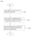
- Embodiment 11 of the invention is next described with reference to Fig. 33.
- Embodiment 11 is a general method of optimizing NMR measurement conditions. Its specific examples are shown in Figs. 34-36.
- NMR measurements are performed while varying a measurement condition to be optimized as shown in Table 28, using the measurement conditions shown in Table 1 and pulse sequence shown in Fig. 1(c).
- Candidates for measurement condition Name of measurement condition Definition
- RF pulse width Time width of certain RF pulse 40
- Frequency of RF pulse FG pulse width Time width of certain magnetic field gradient pulse FG pulse intensity Intensity of certain magnetic field gradient pulse FG pulse shape Shape of certain magnetic field gradient pulse
- Sense of certain magnetic field gradient pulse in absolute coordinate system Wait time Wait time between certain pulses Repeat delay Repetition time Acquisition time Observation time
- Data points Number of sampling points of observed data Total measurement time Time from start to end of measurement
- Lock offset Frequency of lock signal Angle of axis of rotation of sample Angle between axis of rotation of sample tube and static magnetic field in measurement of sample being rotated Sample
- step 2 the measurements data are Fourier-transformed. Then, properties as shown in Table 29 are extracted as numerical values. A curve is created by plotting them along the value varied in step 1.
- Candidates for certain property Property of signal Definition Area Integrated value of signal region Intensity of vertex Intensity of peak top Position of vertex Position of peak top Half-height width Line width at half-peak position Symmetry Left-and-right symmetry, e.g., area ratio of left and right halves on the opposite sides of a peak top
- step 3 curve fitting is done by varying constants of a model equation as shown in Table 30 such that the model equation coincident with the parameter varied in step 1, its range, and the property extracted in step 2 agrees with the curve created in step 2.
- Table 30 x represents the measurement condition varied on the horizontal axis of the graph, and y represents the horizontal axis of the graph and indicates the value of intensity extracted from measurement results under certain measurement conditions.
- a , B, C, D, and E are constants, and they are varied such that the standard deviation ⁇ decreases during curve fitting.
- the step of obtaining an optimum value of a measurement condition does not use visual estimation. Therefore, reproducible results can be obtained.
- Fig. 34 illustrates a first specific example of Embodiment 11.
- This first specific example is a method of optimizing the irradiation center frequency in an NMR measurement.
- step 1 NMR measurements are performed using measurement conditions shown in Table 32 and pulse sequence shown in Fig. 34 (a), for example.
- the center frequency of irradiation is varied about the frequency of signal derived from light water.
- Plural sets of 1D NMR measurement data are obtained.
- step 2 the residual signal derived from light water and indicating the 1D NMR data is Fourier-transformed and integrated values are plotted against the center frequency of irradiation. As a result, a curve as shown in Fig. 34(b) is obtained.
- step 3 the linear least squares method using model equation (16) from which a graph is created is implemented to obtain optimum A, B, and C . Since the optimum center frequency of irradiation is the value of x at the minimum value of the graph of Fig. 34(b), the constants A and B obtained by curve fitting are substituted into Eq. (17), thus obtaining optimum values.
- the pulse sequence is not limited to the sequence shown in Fig. 34(a).
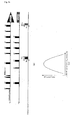
- Fig. 35 illustrates a second specific example of Embodiment 11. A method of optimizing the wait time ⁇ in 15 N- 1 H HSQC is described.
- step 1 1D NMR measurements are performed using measurement conditions as shown in Table 33 and pulse sequence shown in Fig. 35(a), for example, (see Reference 4 ( Chemical Physics Letters, 69, 1980, pp. 185-188), and using varying wait time ⁇ . Thus, plural sets of 1D NMR measurement data are obtained.
- step 2 a certain signal indicating 1D NMR data and derived by Fourier transform is integrated.
- the integrated value is plotted against wait time ⁇ .
- a curve as shown in Fig. 35(b) is obtained.
- step 3 the linear least squares method is implemented using model equation (16) from which a graph is created to obtain optimum A, B, and C . Since the optimum wait time ⁇ is the value of x at the minimum value of the graph of Fig. 35 (b) , the constants A and B obtained by curve fitting are substituted into Eq. (17), thus obtaining optimum values.
- Eq. (16) x indicates the wait time ⁇ and y indicates the integrated value of signal at the wait time x .
- the pulse sequence is not limited to the sequence shown in Fig. 35 (a).
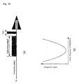
- Fig. 36 illustrates a third specific example of Embodiment 11.
- This third example is a method of optimizing magnetic field gradient pulse intensity Gz 2 in a 15 N- 1 H HSQC (heteronuclear single quantum coherence) measurement (hereinafter simply referred to as SE-HSQC) using coherence selection utilizing magnetic field gradient pulses.
- SE-HSQC heterogeneous single quantum coherence
- step 1 NMR measurements are performed using measurement conditions as shown in Table 34 and pulse sequence shown in Fig. 36 (a) , for example, (see Reference 5 (Journal of the American Chemical Society, 114, 1992, pp. 10663-10665)), and using varying magnetic field gradient pulse intensity Gz 2 . Thus, plural sets of 1D NMR measurement data are obtained.
- step 2 1D NMR data are obtained by Fourier transform, and an integrated value derived from a certain signal contained in the data is obtained. The integrated value is plotted against Gz 2 . As a result, a curve as shown in Fig. 36(b) is obtained.
- step 3 the linear least squares method is implemented using model equation (16) from which a graph is created to obtain optimum A, B, and C . Since the optimum magnetic field gradient pulse intensity Gz 2 is the value of x at the maximum value of the graph of Fig. 36 (b) , the constants A and B obtained by curve fitting are substituted into Eq. (17), thus obtaining optimum values.
- Eq. (16) x indicates the Gz 2 and y indicates the integrated value of signal at the magnetic field gradient pulse intensity x .
- the pulse sequence is not limited to the sequence shown in Fig. 36(a).
- the step of obtaining an optimum value of a measurement condition in an NMR measurement does not include visual estimation. Therefore reproducible results can be obtained. Furthermore, the use of a curve fitting method produces good results even if there are a limited number of data items, as long as they characterize a waveform. Consequently, a reliable optimum value of the measurement condition can be found in a short time.
Landscapes
- Physics & Mathematics (AREA)
- High Energy & Nuclear Physics (AREA)
- Condensed Matter Physics & Semiconductors (AREA)
- General Physics & Mathematics (AREA)
- Magnetic Resonance Imaging Apparatus (AREA)
Abstract
Description
- The present invention relates to a method of optimizing a measurement condition in an NMR measurement.
- Fig. 1 illustrates the prior art method of optimizing an NMR measurement condition. Fig. 1 (a) is a flowchart illustrating a general procedure for finding an optimum value of a measurement condition. Fig. 1 (b) is a flowchart illustrating a procedure for finding optimum values of RF pulse widths. Fig. 1(c) is a diagram illustrating a pulse sequence for measurement of an RF pulse width.
- The general procedure for finding an optimum value of a measurement condition is described by referring to Fig. 1(a). In step 1, NMR measurements are carried out while varying the value of a measurement condition to be optimized in given increments. In step 2, a graph for finding the optimum value from the obtained measurement data by appropriate processing is created. At this time, varying value of the measurement condition is plotted on one axis of the graph. In step 3, the optimum value is found from the shape of the graph by visual estimation.
- As a specific example, a procedure of finding an optimum value of an RF pulse width as a measurement condition is next described by referring to Figs. 1(b) and 1(c). In step 1, NMR measurements are performed while varying the pulse width from 0 to 70 µs using a pulse sequence shown in Fig. 1 (c) , for example, under measurement conditions listed in Table 1.
Measurement condition set 1 under which measurements are performed with varying RF pulse width Item Value Sample 15 mM copper dichloride/1 % H2O, 99%D2O Magnetic field intensity 14.09636928 T Observed nucleus 1H Observe frequency 600.1723046 MHz Center frequency of observation about 4.7 ppm (resonance frequency of water) Number of data points 16384 Sweep width 9.00252071 kHz Number of accumulations 1 B1 pulse intensity about 25 kHz Observation time 1.81993472 s Relaxation_ delay 1 s Temperature 25°C - In the pulse sequence of Fig. 1(c), [relaxation_delay] indicates the wait time of each repetition pulse. In this example, the time is 1 s.
- [x_pulse] indicates an RF pulse. In this example, NMR measurements are performed using a pulse width varied from 0 to 70 µs.
- [acquisition] indicates an observation. In this example, the time necessary for an observation is 1.81993472 s as shown in Table 1.
- Data obtained from a measurement is shown in Fig. 2, where one-dimensional (1D) NMR data obtained using a certain pulse width are arrayed in the order of values of pulse widths at intervals of 2 µs.
- In step 2, the obtained NMR data are first Fourier-transformed. The resulting data are shown in Fig. 3, where the data are arrayed in the order of values of pulse widths at intervals of 2 µs in the same way as in Fig. 2. Then, with respect to each set of 1D NMR data, a range from 4 to 5.5 ppm in the signal region is displayed. The data are arrayed horizontally in the order of values of pulse widths. The obtained graph is shown in Fig. 4, where the horizontal axis indicates the pulse width, while the vertical axis indicates the intensity of the NMR spectrum.
- In step 3, a waveform formed by connecting the vertices of spectral intensities of Fig. 4 by means of straight lines is regarded as a sinusoidal (SIN) wave. Visual estimation of a pulse width of 360° reveals that it is about 28 µs. Since it has been already known that the optimum pulse width is 90°, the optimum pulse width is equal to the pulse width of 360° divided by 4, i.e., 28 µs/4 = 7 µs.
- An NMR instrument designed to quantitatively indicate the nonuniformities in transmit and receive magnetic fields is shown in Patent Reference 1 (Japanese Patent Laid-Open No. H3-139330). In particular, NMR scans are made with RF exciting field intensities of different arrays. A curve is applied to each set of corresponding data elements in one set of intensity arrays. The peaks of the applied curves are determined. Corresponding data in the transmit and receive arrays are generated from the determined peaks. Thus, a magnetic field map indicating nonuniformities in an RF magnetic field by means of the magnitudes of data elements is created.
- However, the prior art method of finding the optimum RF pulse width has the problem that the reliability of the optimum value is low, because the value is found from a created graph by visual estimation. In order to obtain an optimum value with high reliability, it is necessary to increase the number of measurement data items. This prolongs the measurement time. If the number of measurement data items is reduced to shorten the measurement time, the reliability of the obtained optimum value deteriorates.
- Furthermore, Patent Reference 1 does not disclose a technique for optimizing measurement conditions, though the reference discloses a technique quantitatively indicating nonuniformities in transmit and receive fields.
- The present invention is intended to address the foregoing problems. It would be desirable to provide a technique for finding a reliable optimum value of a measurement condition with a reduced number of measurement data items, i.e., in a short time.
- A method of optimizing an NMR measurement condition in accordance with the invention starts with gaining NMR measurement data while varying the value of the measurement condition to be optimized. Then, a certain property is extracted as a numerical value from the measurement data. A plot is made along the varied value of the measurement condition to create a curve. Amodel equation coincident with the measurement condition, its range, and the certain property extracted as a numerical value is established. Curve fitting in which constants of the model equation are varied is done such that the equation agrees with the created curve. Constant values of the model equation and their standard deviation are obtained by curve fitting. An optimum value of the measurement condition is obtained from the results.
- In the present invention, curve fitting is used and so a good result can be obtained if the number of data items is reduced as long as they characterize a waveform. A reliable optimum value of a measurement condition can be found in a short time.
- Other preferred embodiments of the invention will appear in the course of the description thereof, which follows.
-
- Fig. 1 is a diagram illustrating the prior art method of optimizing an NMR measurement condition.
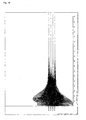
- Fig. 2 is a graph of one-dimensional (1D) NMR data obtained by the method illustrated in Fig. 1.
- Fig. 3 is a graph illustrating data obtained by Fourier-transforming the 1D NMR data shown in Fig. 2.
- Fig. 4 is a graph consisting of pulses having different widths and obtained from the 1D NMR data shown in Fig. 2, and in which the pulse widths are arrayed in the order of their values in a range from 4 to 5.5 ppm.
- Fig. 5 is a flowchart illustrating Embodiment 1 of the invention.
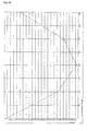
- Fig. 6 is a graph of curves obtained by plotting the integrated values in a given signal region.
- Fig. 7 is a flowchart illustrating Embodiment 2 of the invention.
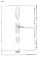
- Fig. 8 is a graph showing NMR measurement data close to 360° pulse width.
- Fig. 9 is a diagram showing data obtained after processing.
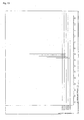
- Fig. 10 is a diagram showing a curve obtained by plotting integrated values.
- Fig. 11 is a flowchart illustrating Embodiment 3 of the invention.
- Fig. 12 is a diagram showing data obtained by a measurement in which an RF pulse width was varied.
- Fig. 13 is a diagram showing data obtained after processing.
- Fig. 14 is a graph showing a curve obtained by plotting integrated values.
- Fig. 15 is a flowchart illustrating Embodiment 4 of the invention.
- Fig. 16 is a diagram showing data obtained by a measurement in which an RF pulse width was varied.
- Fig. 17 is a diagram showing data obtained after processing.
- Fig. 18 is a diagram showing a curve obtained by plotting integrated values.
- Fig. 19 is a flowchart illustrating Embodiment 5 of the invention.
- Fig. 20 is a diagram showing data obtained by a measurement in which an RF pulse width was varied.
- Fig. 21 is a diagram showing data obtained after processing.
- Fig. 22 is a diagram showing a curve obtained by plotting integrated values.
- Fig. 23 is a flowchart illustrating Embodiment 6 of the invention.
- Fig. 24 is a graph showing a curve obtained by plotting peak top intensities.
- Fig. 25 is a flowchart illustrating Embodiment 7 of the invention.
- Fig. 26 is a graph showing a curve obtained by plotting peak top intensities.
- Fig. 27 is a flowchart illustrating Embodiment 8 of the invention.
- Fig. 28 is a graph showing a curve obtained by plotting peak top intensities.
- Fig. 29 is a flowchart illustrating Embodiment 9 of the invention.
- Fig. 30 is a graph showing a curve obtained by plotting peak top intensities.
- Fig. 31 is a flowchart illustrating Embodiment 10 of the invention.
- Fig. 32 is a graph showing a curve obtained by plotting peak top intensities.
- Fig. 33 is a flowchart illustrating Embodiment 11 of the invention.
- Fig. 34 is a diagram illustrating a first specific example of Embodiment 11.
- Fig. 35 is a diagram illustrating a second specific example of Embodiment 11.
- Fig. 36 is a diagram illustrating a third specific example of Embodiment 11.
-
- The preferred embodiments of the present invention are hereinafter described. Of the following embodiments, Embodiments 1-5 pertain to a method of finding an optimum value of an RF pulse width using integrated values in the signal region. Embodiments 6-10 pertain to a method of finding an optimum value of an RF pulse width using peak top intensities of a signal. In the following description, the measurement conditions of Table 1 and the pulse sequence of Fig. 1(c) are used. Of course, the invention is not restricted to the measurement conditions of Table 1 and pulse sequence of Fig. 1 (c) . Embodiment 11 pertains to a general method of optimizing an NMR measurement condition. In the following description, the unit name "abn" in the various tables is identical with the unit name "au" and means a unitless intensity or magnitude.
- Fig. 5 is a flowchart illustrating Embodiment 1 of the invention. (a) of Fig. 5 illustrates a procedure for finding an optimum value of an RF pulse width. (b) of Fig. 5 illustrates a procedure for finding an initial value in a DFP method (described later) . Embodiment 1 is a method of finding an optimum RF pulse width by measuring the pulse width over the whole range.
- In Fig. 5 (a) , in step 1, NMR measurements are performed while varying an RF pulse width from 0 to 70 µs in increments of 2 µs, using the measurement conditions shown in Table 1 and pulse sequence shown in Fig. 1 (c) , for example. As a result, measurement data shown in Fig. 2 are obtained.
- In step 2, the measurement data are Fourier-transformed, and a plot is done along the values of the RF pulse width using integrated values in the signal region. In this way, a curve is created. This processing results in data as shown in Fig. 3. Finding the integrated values from a signal range from 4 to 5.5 ppm produces results listed in Table 2. Plotting the results gives rise to the curve indicated by the solid line in Fig. 6.
Results 1 of calculations of integrated values Index x_90_width Intensity 1 0 µs -3.9417 kabn 2 2 µs 50.35382 Mabn 3 4 µs 96.74335 Mabn 4 6 µs 126.74086 Mabn 5 8 µs 134.78419 Mabn 6 10 µs 119.99778 Mabn 7 12 µs 84.80437 Mabn 8 14 µs 37.11067 Mabn 9 16 µs -14.37721 Mabn 10 18 µs -60.44845 Mabn 11 20 µs -93.60701 Mabn 12 22 µs -106.62882 Mabn 13 24 µs -98.13594 Mabn 14 26 µs -70.18078 Mabn 15 28 µs -28.46294 Mabn 16 30 µs 18.92854 Mabn 17 32 µs 61.74452 Mabn 18 34 µs 93.01865 Mabn 19 36 µs 105.83569 Mabn 20 38 µs 98.68427 Mabn 21 40 µs 72.78549 Mabn 22 42 µs 34.93452 Mabn 23 44 µs -7.80636 Mabn 24 46 µs -45.95444 Mabn 25 48 µs -76.29246 Mabn 26 50 µs -90.08089 Mabn 27 52 µs -84.6685 Mabn 28 54 µs -62.78815 Mabn 29 56 µs -28.93477 Mabn 30 58 µs 10.14414 Mabn 31 60 µs 47.04411 Mabn 32 62 µs 73.08897 Mabn 33 64 µs 85.13906 Mabn 34 66 µs 80.43171 Mabn 35 68 µs 60.11846 Mabn 36 70 µs 29.17292 Mabn - In step 3, curve fitting (described later) is performed in which the constants A, B, C, D, and ω of model equation (1) (given later) are varied such that model equation (1) agrees with the curve indicated by the solid line in Fig. 6. Model equation (1) (Eq. (1)), Eq. (2) for finding a 360° RF pulse width, and Eq. (3) for finding a 90° RF pulse width are given below.

- Curve fitting using model equation (1) produces results shown in Table 3.
Results 1 of calculations of curve fitting Constant Value A 120149.01181 kabn B 0 rad C 207.85512 µs D 5381.92103 kabn ω 0.21696 rad/µs σ 9792.45099 kabn - Plotting of the values of Table 3 using model equation (1) produces the curve indicated by the broken line in Fig. 6, thus obtaining the constant values A, B, C, D, and ω and their standard deviation σ. Substituting the results into Eq. (2) gives rises to 360° pulse width (PW360) = 28.96043 µs. This is substituted into Eq. (3), resulting in PW90 = 7.24011 µs that is an optimum RF pulse width. The standard deviation σ in Table 3 gives an index of the reliability of the obtained RF pulse width.
- Curve fitting is to find the A, B, C, D, and ω which minimize the following evaluation formula (4) using a multi-dimensional variable metric method (Davidon-Fletcher-Powell (DFP) method) described herein as Reference 1 (Numerical Recipes in C: THE ART OF SCIENTIFIC COMPUTING, Second Edition (ISEN 0-521-43108-5), 1992, pp. 425-430) . The DFP method needs an evaluation equation and initial values. Eq. (4) using Eq. (5) identical with Eq. (1) is employed as this evaluation formula.


- In Eq. (4) , t is an RF pulse width, PWstart is the start value of the RF pulse width, PWend is the end value of the width, and g(t) is the actually measured value of the intensity at the RF pulse width of t. The theoretical value f(t) of intensity is defined by Eq. (5) and equal to the right side of Eq. (1).
- A method of finding the initial values used in the DFP method is next described with reference to Fig. 5 (b) . In step 1, the initial values of ω and C of model equation (1) are computed using the LPSVD (Linear Prediction Singular Value Deconvolution) method that indicates a method of finding the initial values (Reference 2 (Journal of Magnetic Resonance, 61, 1985, pp. 465-481) . If calculations using the LPSVD method are successful, initial values ω = 0.21703 rad/µs and C = 231.59569 µs are obtained.
- In step 2, if calculations using the LPSVD method are unsuccessful, the program goes to step 3. If the calculations are successful, the program goes to step 7.
- In step 3, the number n1 of passes of the curve indicated by the solid line in Fig. 6 across straight line y = 0 and the RF pulse widths zp[1] , ... , zp [n1] at this time are found. The results are shown in Table 4.
Intersection 1 with y = 0 Item Value n1 5 zp[1] 0.00016 µs zp[2] 15.44153 µs zp[3] 29.20118 µs zp[4] 43.63471 µs zp[5] 57.48084 µs - In step 4, the results shown in Table 4 are substituted into Eq. (6). As an initial value of ω, we obtain ω = 0.21862 rad/µs.
- In step 5, the number of positive-going (upward) peaks n2 of the curve indicated by the solid line in Fig. 6, the RF pulse widths pp[1], .., pp[n2] at the tops of the peaks, and the intensities pi [1] , ..., pi[n2] of the tops of the peaks are found. The results are listed in Table 5.
Tops 1 of peaks Item Value n2 3 pp[1] 8 µs pp[2] 36 µs pp[3] 64 µs pi[1] 134.78419 kabn pi[2] 105.83569 kabn pi[3] 85.13906 kabn - In step 6, the results shown in Table 5 are substituted into Eq. (7). We obtain 121.90106 µs as an initial value of C (C= 121.90106 µs).

- In step 7, the values of ω and C calculated in step 1 or steps 4 and 6 are substituted into Eq. (8) that is an expansion of Eq. (5). Using each item as a basis function and employing the curve indicated by the solid line in Fig. 6, the linear least squares method shown in Reference 3 (Numerical Recipes in C: THE ART OF SCIENTIFIC COMPUTING, Second Edition (ISEN 0-521-43108-5), 1992, pp. 671-681) is implemented. Results (optimum constant values D, E, and F) listed in Table 6 are obtained. Table 6 uses the results of step 1.

Results 1 of calculations of linear least squares method Item Value D 5381.95203 kabn E 119968.83441 kabn F -6577.86175999999 kabn - In step 8, the results shown in Table 6 are substituted into calculation formulas (9), (10-1), and (10-2), resulting in A = 120149.03035 kabn and B = 0.05477 rad.
- Then, ω and C calculated in step 1 or steps 4 and 6, D calculated in step 7, and A and B calculated in step 8 are used as initial values in the DFP method. These values are varied. The values of A, B, C, D, and ω that minimize the value of evaluation formula (4) are found. Where the initial values of the DFP method are used, if measurement conditions as listed in Table 1 and the pulse sequence shown in Fig. 1(c), for example, are used, it is known that B = 0 rad. Therefore, the DFP method is so implemented that the constants A, C, D, and ω are varied while the constant B of model equation (1) is kept at 0 rad.
- In the present embodiment, the step of obtaining an optimum RF pulse width contains no manual operation and so reproducible results can be obtained. In the above description, the number of data items is set equal to the number of data items used in the prior art procedure for convenience of illustration. In curve fitting, in a case where there are data points characterizing a waveform, if the number of data points is reduced, similar results can be obtained. Therefore, good results can be obtained if there are a reduced number of data items. This similarly applies to embodiments described later.
- Embodiment 2 of the invention is described next with reference to Fig. 7. Embodiment 2 is a method of finding an optimum RF pulse width by performing NMR measurements while varying the pulse width in the neighborhood of 360° pulse width. In the following description, it is assumed that it is previously known that the 360° pulse width is 28 µs because of the technique described as the prior art or information obtained from other technique.
- In step 1, NMR measurements are performed while varying an RF pulse width from 24 to 34 µs (i.e., around 360° pulse width) in increments of 2 µs, using the measurement conditions shown in Table 1 and pulse sequence shown in Fig. 1 (c) , for example. Measurement data shown in Fig. 8 are obtained.
- In step 2, the measurement data are Fourier-transformed, and integrated values in the signal region are plotted along the values of the RF pulse width. In this way, a curve is created. This processing results in data shown in Fig. 9. Finding the integrated values from a signal range from 4 to 5.5 ppm produces results listed in Table 7. Plotting the results gives rise to the curve indicated by the solid line in Fig. 10.
Results 2 of calculations of integrated values Index x_90_width Intensity 1 24 µs -49.11459 Mabn 2 26 µs -35.15117 Mabn 3 28 µs -14.27532 Mabn 4 30 µs 9.45965 Mabn 5 32 µs 30.95036 Mabn 6 34 µs 46.61799 Mabn - In step 3, the linear least squares method is implemented using model equation (11). Results shown in Table 8 are obtained. Plotting of the contents of Table 8 using model equation (11) results in the curve indicated by the broken line in Fig. 10.
Results 2 of calculations of curve fitting Constant Value A 10.01003 Mabn/µs B -292.20986 Mabn σ 2.68816 Mabn - Then, the values in Table 8 are substituted into Eq. (12), producing PW360 = 29.19169 µs as a 360° pulse. This is substituted into Eq. (3) , giving rise to an optimum RF pulse width PW90 = 7.29792 µs. The standard deviation σ in Table 8 gives an index of the reliability of the obtained RF pulse width.
- In the present embodiment, the step of obtaining the RF pulse width does not use visual estimation. Therefore, reproducible results can be obtained.
- Embodiment 3 of the invention is next described with reference to Fig. 11. Embodiment 3 is a method of finding an optimum RF pulse width by performing NMR measurements while varying the pulse width in the neighborhood of 90° pulse width. In the following description, it is assumed that it is previously known that the 90° pulse width is 7 µs because of the technique described as the prior art or information obtained from other technique.
- In step 1, NMR measurements are performed while varying an RF pulse width from 4 to 12 µs (i.e., around 90° pulse width) in increments of 2 µs, using the measurement conditions shown in Table 1 and pulse sequence shown in Fig. 1(c), for example. Measurement data shown in Fig. 12 are obtained.
- In step 2, the measurement data are Fourier-transformed, and integrated values in the signal region are plotted along the values of the RF pulse width. In this way, a curve is created. This processing results in data shown in Fig. 13. Finding the integrated values from a signal existing region from 4 to 5.5 ppm produces results listed in Table 9. Plotting the results gives rise to the curve indicated by the solid line in Fig. 14.
Results 3 of calculations of integrated values Index x_90_width Intensity 1 4 µs 48.48201 Mabn 2 6 µs 63.54521 Mabn 3 8 µs 67.35346 Mabn 4 10 µs 60.167 Mabn 5 12 µs 42.88578 Mabn - In step 3, the linear least squares method is implemented using model equation (13). Results shown in Table 10 are obtained. Plotting of the contents of Table 10 using model equation (13) results in the curve indicated by the broken line in Fig. 14.
Results 3 of calculations of curve fitting Constant Value A -1.35149 Mabn/µs2 B 20.89533 Mabn/µs C -13.36858 Mabn σ 0.18738 Mabn - Then, the values in Table 10 are substituted into Eq. (12), producing PW90 = 7.73047 µs as an optimum RF pulse width. The standard deviation σ in Table 10 gives an index of the reliability of the obtained RF pulse width.
- In the present embodiment, the step of obtaining the RF pulse width does not use visual estimation. Therefore, reproducible results can be obtained.
- Embodiment 4 of the invention is next described with reference to Fig. 15. Embodiment 4 is a method of finding an optimum RF pulse width by performing NMR measurements while varying the pulse width in the neighborhood of 180° pulse width. In the following description, it is assumed that it is previously known that the 180° pulse width is 14 µs because of the technique described as the prior art or information obtained from other technique.
- In step 1, NMR measurements are performed while varying an RF pulse width from 12 to 18 µs (i.e., around 180° pulse width) in increments of 2 µs, using the measurement conditions shown in Table 1 and pulse sequence shown in Fig. 1 (c) , for example. Measurement data shown in Fig. 16 are obtained.
- In step 2, the measurement data are Fourier-transformed, and integrated values in the signal region are plotted along the values of the RF pulse width. In this way, a curve is created. This processing results in data shown in Fig. 17. Finding the integrated values from a signal existing range from 4 to 5.5 ppm produces results listed in Table 11. Plotting the results gives rise to the curve indicated by the solid line in Fig. 18.
Results 4 of calculations of integrated values Index x_90_width Intensity 1 12 µs 42.88578 Mabn 2 14 µs 18.76097 Mabn 3 16 µs -7.33509 Mabn 4 18 µs -30.59374 Mabn - In step 3, the linear least squares method is implemented using model equation (11). Results shown in Table 12 are obtained. Plotting of the contents of Table 12 using model equation (11) results in the curve indicated by the broken line in Fig. 19.
Results 4 of calculations of curve fitting Constant Value A -12.32673 Mabn/µs B 190.83045 Mabn σ 0.66926 Mabn - Then, the values in Table 12 are substituted into Eq. (14), producing PW90 = 7.74051 µs as an optimum RF pulse width. The standard deviation σ in Table 12 gives an index of the reliability of the obtained RF pulse width. In the present embodiment, the step of obtaining the RF pulse width does not use visual estimation. Therefore, reproducible results can be obtained.
- Embodiment 5 of the invention is next described by referring to Fig. 19. Embodiment 5 is a method of finding an optimum RF pulse width by performing NMR measurements while varying the pulse width in the neighborhood of 270° pulse width. In the following description, it is assumed that it is previously known that the 270° pulse width is 21 µs because of the technique described as the prior art or information obtained from other technique.
- In step 1, NMR measurements are performed while varying an RF pulse width from 18 to 26 µs (i.e., around 270° pulse width) in increments of 2 µs, using the measurement conditions shown in Table 1 and pulse sequence shown in Fig. 1 (c) , for example. Measurement data shown in Fig. 20 are obtained.
- In step 2, the measurement data are Fourier-transformed, and integrated values in the signal region are plotted along the values of the RF pulse width. In this way, a curve is created. This processing results in data shown in Fig. 21. Finding the integrated values from a signal existing region from 4 to 5.5 ppm produces results listed in Table 13. Plotting the results gives rise to the curve indicated by the solid line in Fig. 22.
Results 5 of calculations of integrated values Index x_90_width Intensity 1 18 µs -30.59374 Mabn 2 20 µs -47.13169 Mabn 3 22 µs -53.43675 Mabn 4 24 µs -49.11459 Mabn 5 26 µs -35.15117 Mabn - In step 3, the linear least squares method is implemented using model equation (13). Results shown in Table 14 are obtained. Plotting of the contents of Table 14 using model equation (13) results in the curve indicated by the broken line in Fig. 22.
Results 5 of calculations of curve fitting Constant Value A 1.27911 Mabn/µs2 B -56.83557 Mabn/µs C 577.97661 Mabn σ 0.12472 Mabn - Then, the values in Table 14 are substituted into Eq. (15), producing PW90 = 7.40563 µs as an optimum RF pulse width. The standard deviation σ in Table 14 gives an index of the reliability of the obtained RF pulse width.
- In the present embodiment, the step of obtaining the RF pulse width does not use visual estimation. Therefore, reproducible results can be obtained.
- Embodiment 6 of the invention is described with reference to Fig. 23. Embodiment 6 is a method of finding an optimum RF pulse width by performing NMR measurements while varying the pulse width in a range from 0 to 360° and using peak top intensities of a signal.
- In step 1, NMR measurements are performed while varying an RF pulse width from 0 to 70 µs in increments of 2 µs, using the measurement conditions shown in Table 1 and pulse sequence shown in Fig. 1(c), for example. Measurement data shown in Fig. 2 are obtained.
- In step 2, the measurement data are Fourier-transformed, and the top intensities of maximum peaks in the signal region are plotted along the values of the RF pulse width. This processing results in data as shown in Fig. 3. Finding the maximum peak top intensities in the signal existing region from 4 to 5.5 ppm produces results listed in Table 15. Plotting the results gives rise to the curve indicated by the solid line in Fig. 24.
Results 1 of calculations of peak top intensities Index x_90_width Intensity 1 0 µs -686.46028 abn 2 2 µs 1.432 Mabn 3 4 µs 2.91449 Mabn 4 6 µs 4.23296 Mabn 5 8 µs 5.27167 Mabn 6 10 µs 5.79026 Mabn 7 12 µs 5.3959 Mabn 8 14 µs 2.91626 Mabn 9 16 µs -2.4162 Mabn 10 18 µs -4.82156 Mabn 11 20 µs -5.28899 Mabn 12 22 µs -4.76431 Mabn 13 24 µs -3.77162 Mabn 14 26 µs -2.49942 Mabn 15 28 µs -1.0764 Mabn 16 30 µs 491.43929 Mabn 17 32 µs 1.87553 Mabn 18 34 µs 3.17844 Mabn 19 36 µs 4.16982 Mabn 20 38 µs 4.73415 Mabn 21 40 µs 4.49485 Mabn 22 42 µs 2.71549 Mabn 23 44 µs -1.14449 Mabn 24 46 µs -3.60914 Mabn 25 48 µs -4.42519 Mabn 26 50 µs -4.20325 Mabn 27 52 µs -3.41928 Mabn 28 54 µs -2.343 Mabn 29 56 µs -1.08743 Mabn 30 58 µs 339.72675 Mabn 31 60 µs 1.5567 Mabn 32 62 µs 2.65856 Mabn 33 64 µs 3.52513 Mabn 34 66 µs 3.94934 Mabn 35 68 µs 3.63341 Mabn 36 70 µs 2.05146 Mabn - In step 3, a curve fitting DFP method is performed in which the constants A, B, C, D, and ω of model equation (1) are varied such that model equation (1) agrees with the curve. Consequently, results shown in Table 16 are obtained.
Results 6 of calculations of curve fitting Constant Value A 5780247.97088 abn B 0 rad C 165.63334 µs D 12119.0114 abn ω 0.21641 rad/µs σ 964882.75674 abn - Plotting of the values of Table 16 using model equation (1) produces the curve indicated by the broken line in Fig. 24. Substituting the values in Table 16 into Eq. (2) gives rises to PW360 = 29.03433 µs. This is substituted into Eq. (3), resulting in PW90 = 7.25858 µs as an optimum RF pulse width. The standard deviation σ in Table 16 gives an index of the reliability of the obtained RF pulse width.
- The method of finding the initial values of A, B, C, D, and ω in the curve fitting DFP method is the same as the method illustrated in Fig. 5 (b). Accordingly, the procedure is described with reference to the flowchart of Fig. 5(b).
- In step 1, the LPSVD method is used but calculations are unsuccessfully performed with no results. The program goes to step 3, where the number of times n1 that the curve indicated by the solid line in Fig. 24 crosses straight line y = 0 is found. Also, the RF pulse widths zp[1], ..., zp[n1] produced at this time are found. Results shown in Table 17 are obtained.
Intersection 2 with y = 0 Item Value n1 5 zp[1] 0.00096 µs zp[2] 15.09378 µs zp[3] 29.3731 µs zp[4] 43.407 µs zp[5] 57.52391 µs - In step 4, the results shown in Table 17 are substituted into Eq. (6). As an initial value of ω, we obtain ω = 0.21846 rad/µs.
- In step 5, the number of positive-going (upward) peaks n2 of the curve indicated by the solid line of Fig. 24, the RF pulse widths pp [1] , .., pp [n2] at the tops of the peaks, and the intensities pi [1] , ..., pi [n2] of the tops of the peaks are found. Results listed in Table 18 are obtained.
Tops 2 of peaks Item Value n2 3 pp[1] 10 µs pp[2] 38 µs pp[3] 66 µs pi[1] 5.79026 Mabn pi[2] 4.73415 Mabn pi[3] 3.94934 Mabn - In step 6, the results shown in Table 18 are substituted into Eq. (7). We obtain C = 146.35619 µs as an initial value of C.
- In step 7, the values of ω and C calculated in steps 4 and 6 are substituted into Eq. (8). Using each item as a basis function and employing the curve indicated by the solid line in Fig. 24, the linear least squares method is implemented. Results (optimum constant values D, E, and F) listed in Table 19 are obtained.
Results 2 of calculations of linear least squares method Item Value D 46209.1885 abn E 5919590.1939 abn F -796281.22262 abn - In step 8, the results shown in Table 19 are substituted into Eqs. (9), (10-1), and (10-2), resulting in A = 5972906.48254 abn and B = 0.13371 rad.
- The values calculated in this way are taken as initial values in the DFP method. These values are varied. The values of A, B, C, D, and ω that minimize the value of evaluation formula (4) are found. Where the initial values of the DFP method are used, in a case where measurement conditions as listed in Table 1 and the pulse sequence shown in Fig. 1 (c) are used, for example, it is known that B = 0 rad. Therefore, the DFP method is so implemented that the constants A, C, D, and ω are varied while the constant B of model equation (1) is kept at 0 rad.
- In the present embodiment, the step of obtaining an optimum RF pulse width contains no manual operation and so reproducible results can be obtained.
- Embodiment 7 of the invention is described by referring to Fig. 25. Embodiment 7 is a method of finding an optimum RF pulse width by performing NMR measurements while varying the RF pulse width in the neighborhood of 360° pulse width. In the following description, it is assumed that it is previously known that the 360° pulse width is 28 µs because of the technique described as the prior art or information obtained from other technique.
- In step 1, NMR measurements are performed while varying an RF pulse width from 24 to 34 µs (i.e., around 360° pulse width) in increments of 2 µs, using the measurement conditions shown in Table 1 and pulse sequence shown in Fig. 1(c), for example. Measurement data shown in Fig. 8 are obtained.
- In step 2, the measurement data are Fourier-transformed, and the top intensities of maximum peaks in the signal region are plotted along the values of the RF pulse width. This processing results in data as shown in Fig. 9. Finding the top intensities of maximum peaks in a signal existing region from 4 to 5.5 ppm produces results listed in Table 20. Plotting the results gives rise to the curve indicated by the solid line in Fig. 26.
Results 2 of calculations of peak top intensities Index x_90_width Intensity 1 24 µs -5.96076 Mabn 2 26 µs -3.78569 Mabn 3 28 µs -1.6393 Mabn 4 30 µs 873.45073 kabn 5 32 µs 2.8408 Mabn 6 34 µs 4.99155 Mabn - In step 3, the linear least squares method is implemented using model equation (11). Results shown in Table 21 are obtained. Plotting of the contents of Table 21 using model equation (11) results in the curve indicated by the broken line in Fig. 26.
Results 7 of calculations of curve fitting Constant Value A 1.1022 Mabn/µs B -32.41038 Mabn σ 0.11171 Mabn - Then, the values in Table 21 are substituted into Eq. (12), producing PW360 = 29.40524 µs. This is substituted into Eq. (3), giving rise to PW90 = 7.35131 µs as an optimum RF pulse width. The standard deviation σ in Table 21 gives an index of the reliability of the obtained RF pulse width.
- In the present embodiment, the step of obtaining an optimum RF pulse width does not use visual estimation. Therefore, reproducible results can be obtained.
- Embodiment 8 of the invention is next described with reference to Fig. 27. Embodiment 8 is a method of finding an optimum RF pulse width by performing NMR measurements while varying the RF pulse width in the neighborhood of 90° pulse width and by using the peak top intensities of the signal. In the following description, it is assumed that it is previously known that the 90° pulse width is 7 µs because of the technique described as the prior art or information obtained from other technique.
- In step 1, NMR measurements are performed while varying an RF pulse width from 4 to 12 µs (i.e., around 90° pulse width) in increments of 2 µs, using the measurement conditions shown in Table 1 and pulse sequence shown in Fig. 1(c). Measurement data shown in Fig. 12 are obtained.
- In step 2, the measurement data are Fourier-transformed, and the top intensities of the maximum peaks in the signal region are plotted along the values of the RF pulse width. This processing results in data shown in Fig. 13. Finding the top intensities of the maximum peaks in a signal existing range from 4 to 5.5 ppm produces results listed in Table 22. Plotting the results gives rise to the curve indicated by the solid line in Fig. 28.
Results 3 of calculations of peak top intensities Index x_90_width Intensity 1 4 µs 4.27768 Mabn 2 6 µs 6.43286 Mabn 3 8 µs 8.34666 Mabn 4 10 µs 9.39558 Mabn 5 12 µs 10.03132 Mabn - In step 3, the linear least squares method is implemented using model equation (13). Results shown in Table 23 are obtained. Plotting of the contents of Table 23 using model equation (13) results in the curve indicated by the broken line in Fig. 28.
Results 8 of calculations of curve fitting Constant Value A -0.069719 Mabn/µs2 B 1.83886 Mabn/µs C -1.99495 Mabn σ 0.06976 Mabn - Then, the values in Table 23 are substituted into Eq. (14), producing PW90 = 13.18934 µs as an optimum RF pulse width. The standard deviation σ in Table 12 gives an index of the reliability of the obtained RF pulse width.
- In the present embodiment, the step of obtaining the optimum RFpulse width does not use visual estimation. Therefore, reproducible results can be obtained.
- Embodiment 9 of the invention is described by referring to Fig. 29. Embodiment 9 is a method of finding an optimum RF pulse width by performing NMR measurements while varying the RF pulse width in the neighborhood of 180° pulse width and using the peak top intensities of the signal. In the following description, it is assumed that it is previously known that the 180° pulse width is 14 µs because of the technique described as the prior art or information obtained from other technique.
- In step 1, NMR measurements are performed while varying an RF pulse width from 12 to 18 µs (i.e., around 180° pulse width) in increments of 2 µs, using the measurement conditions shown in Table 1 and pulse sequence shown in Fig. 1(c), for example. Measurement data shown in Fig. 16 are obtained.
- In step 2, the measurement data are Fourier-transformed, and the top intensities of the maximum peaks in the signal region are plotted along the values of the RF pulse width. This processing results in data as shown in Fig. 17. Finding the peak top intensities of the maximum peaks in a signal existing range from 4 to 5.5 ppm produces results listed in Table 24. Plotting the results gives rise to the curve indicated by the solid line in Fig. 30.
Results 4 of calculations of peak top intensities Index x_90_width Intensity 1 12 µs 10.03132 Mabn 2 14 µs 7.52695 Mabn 3 16 µs -6.83314 Mabn 4 18 µs -9.34702 Mabn - In step 3, the linear least squares method is implemented using model equation (11). Results shown in Table 25 are obtained. Plotting of the contents of Table 25 using model equation (11) results in the curve indicated by the broken line in Fig. 30.
Results 9 of calculations of curve fitting Constant Value A -3.62476 Mabn/µs B 54.71586 Mabn σ 3.05991 Mabn - Then, the values in Table 25 are substituted into Eq. (14), producing PW90 = 7.54752 µs as an optimum RF pulse width. The standard deviation σ in Table 25 gives an index of the reliability of the obtained RF pulse width. In the present embodiment, the step of obtaining the optimum RF pulse width does not use visual estimation. Therefore, reproducible results can be obtained.
- Embodiment 10 of the invention is described by referring to Fig. 31. Embodiment 10 is a method of finding an optimum RF pulse width by performing NMR measurements while varying the RF pulse width in the neighborhood of 270° pulse width and by using the peak top intensities of the signal. In the following description, it is assumed that it is previously known that the 270° pulse width is 21 µs because of the technique described as the prior art or information obtained from other technique.
- In step 1, NMR measurements are performed while varying an RF pulse width from 18 to 26 µs (i.e., around 270° pulse width) in increments of 2 µs, using the measurement conditions shown in Table 1 and pulse sequence shown in Fig. 1 (c) , for example. Measurement data shown in Fig. 20 are obtained.
- In step 2, the measurement data are Fourier-transformed, and the top intensities of the maximum peaks in the signal region are plotted along the values of the RF pulse width. This processing results in data as shown in Fig. 21. Finding the top intensities of the maximum peaks in a signal existing region from 4 to 5.5 ppm produces results listed in Table 26. Plotting the results gives rise to the curve indicated by the solid line in Fig. 32.
Results 5 of calculations of peak top intensities Index x_90_width Intensity 1 18 µs -9.34702 Mabn 2 20 µs -9.03598 Mabn 3 22 µs -7.89824 Mabn 4 24 µs -5.96076 Mabn 5 26 µs -3.78569 Mabn - In step 3, the linear least squares method is implemented using model equation (13). Results shown in Table 27 are obtained. Plotting of the contents of Table 27 using model equation (13) results in the curve indicated by the broken line in Fig. 32.
Results 10 of calculations of curve fitting Constant Value A 0.08085 Mabn/µs2 B -2.84765 Mabn/µs C 15.66296 Mabn σ 0.09848 Mabn - Then, the values in Table 27 are substituted into Eq. (15), producing PW90 = 5.87 µs as an optimum RF pulse width. The standard deviation σ in Table 27 gives an index of the reliability of the obtained RF pulse width.
- In the present embodiment, the step of obtaining the optimum RF pulse width does not use visual estimation. Therefore, reproducible results can be obtained.
- Embodiment 11 of the invention is next described with reference to Fig. 33. Embodiment 11 is a general method of optimizing NMR measurement conditions. Its specific examples are shown in Figs. 34-36.
- In step 1, NMR measurements are performed while varying a measurement condition to be optimized as shown in Table 28, using the measurement conditions shown in Table 1 and pulse sequence shown in Fig. 1(c).
Candidates for measurement condition Name of measurement condition Definition RF pulse width Time width of certain RF pulse 40 Intensity of certain RF pulse
Phase of certain RF pulseRF pulse shape Shape of certain RF pulse RF offset Frequency of RF pulse FG pulse width Time width of certain magnetic field gradient pulse FG pulse intensity Intensity of certain magnetic field gradient pulse FG pulse shape Shape of certain magnetic field gradient pulse Direction of application of FG pulse Sense of certain magnetic field gradient pulse in absolute coordinate system Wait time Wait time between certain pulses Repeat delay Repetition time Acquisition time Observation time Scan Number of repetitions Sweep width Width of observe frequency Data points Number of sampling points of observed data Total measurement time Time from start to end of measurement Lock offset Frequency of lock signal Angle of axis of rotation of sample Angle between axis of rotation of sample tube and static magnetic field in measurement of sample being rotated Sample temperature Temperature of sample under measurement Pressure Pressure inside sample tube Spin rate Spin rate of sample tube Volume Volume of sample pH pH of sample Concentration Concentration of sample Position Position of sample tube Static magnetic field intensity Intensity of static magnetic field on sample Flow rate Flow rate of sample through cell in LC-NMR probe Q value Q value of transmit/receive circuit of probe Shim value Current value of shim coil Room temperature Temperature of measuring chamber Coil length Length of probe coil Filter characteristics Parameters determining characteristics of digital and analog filters Length of cable Length of cable used in portions associated with NMR measurement such as NMR spectrometer and probe Thickness of cable Thickness of cable used in portions associated with NMR measurement such as NMR spectrometer and probe - In step 2, the measurements data are Fourier-transformed. Then, properties as shown in Table 29 are extracted as numerical values. A curve is created by plotting them along the value varied in step 1.
Candidates for certain property Property of signal Definition Area Integrated value of signal region Intensity of vertex Intensity of peak top Position of vertex Position of peak top Half-height width Line width at half-peak position Symmetry Left-and-right symmetry, e.g., area ratio of left and right halves on the opposite sides of a peak top - In step 3, curve fitting is done by varying constants of a model equation as shown in Table 30 such that the model equation coincident with the parameter varied in step 1, its range, and the property extracted in step 2 agrees with the curve created in step 2. In Table 30, x represents the measurement condition varied on the horizontal axis of the graph, and y represents the horizontal axis of the graph and indicates the value of intensity extracted from measurement results under certain measurement conditions. A, B, C, D, and E are constants, and they are varied such that the standard deviation σ decreases during curve fitting.

- Values of the constants and their standard deviation are obtained by this curve fitting. From these results, an optimum value of a measurement condition as shown in Table 31 is obtained. The standard deviation σ gives an index of the reliability of the obtained optimum value.
Candidates for optimum value Optimum value Definition Maximum x Value of x when the intensity of graph (value on vertical axis) maximizes Minimum x Value of x when the intensity of graph (value on vertical axis) minimizes x equal to 0 Value of x when the intensity of graph (value on vertical axis) approaches closest to 0 Results of calculation of constant value Value obtained from calculation formula, using an optimum constant value derived as a result of curve fitting as described in Embodiments 1-10 - In the present embodiment, the step of obtaining an optimum value of a measurement condition does not use visual estimation. Therefore, reproducible results can be obtained.
- Fig. 34 illustrates a first specific example of Embodiment 11. This first specific example is a method of optimizing the irradiation center frequency in an NMR measurement.
- In step 1, NMR measurements are performed using measurement conditions shown in Table 32 and pulse sequence shown in Fig. 34 (a), for example. The center frequency of irradiation is varied about the frequency of signal derived from light water. Plural sets of 1D NMR measurement data are obtained.
Measurement conditions for optimization of center frequency of irradiation Item Value Sample 1 mM albumen lysozyme/90% H20, 10% D2O Magnetic field intensity 14.09636928 T Observed nucleus 1H Observe frequency 600.1723046 MHz Observation center frequency Center frequency of irradiation Number of data points 16384 Sweep width 9.00252071 kHz Number of accumulations 1 Pulse width 1 µs B1 pulse intensity 25 kHz Saturation power 0.25 kHz Saturation delay 2 s Observation time 1.81993472 s relaxation_delay 1 s Temperature 25°C - In step 2, the residual signal derived from light water and indicating the 1D NMR data is Fourier-transformed and integrated values are plotted against the center frequency of irradiation. As a result, a curve as shown in Fig. 34(b) is obtained.
- In step 3, the linear least squares method using model equation (16) from which a graph is created is implemented to obtain optimum A, B, and C. Since the optimum center frequency of irradiation is the value of x at the minimum value of the graph of Fig. 34(b), the constants A and B obtained by curve fitting are substituted into Eq. (17), thus obtaining optimum values. In the present specific example, the pulse sequence is not limited to the sequence shown in Fig. 34(a).
- Fig. 35 illustrates a second specific example of Embodiment 11. A method of optimizing the wait time δ in 15N-1H HSQC is described.
- In step 1, 1D NMR measurements are performed using measurement conditions as shown in Table 33 and pulse sequence shown in Fig. 35(a), for example, (see Reference 4 (Chemical Physics Letters, 69, 1980, pp. 185-188), and using varying wait time δ. Thus, plural sets of 1D NMR measurement data are obtained.
Measurement conditions for optimization of wait time δ in 15N-1H HSQC Item Value Sample 1 mM 15N labelled ubiquitin/90% H2O, 10% D2O Magnetic field intensity 14.09636928 T Observed nucleus 1H Irradiating nucleus 15N Observe frequency 600.1723046 MHz Observation center frequency about 4.7 ppm (resonance frequency of water) Number of data points 512 Sweep width 9.00252071 kHz Number of accumulations 2 Pulse width 10µs 1HB1 pulse intensity 25 kHz 15 NB1 pulse intensity 6.25 kHz 15N decoupled B1 pulse intensity 0.78 kHz t1 1 µs Observation time 57 ms relaxation_delay 1 s Temperature 25°C - In step 2, a certain signal indicating 1D NMR data and derived by Fourier transform is integrated. The integrated value is plotted against wait time δ. As a result, a curve as shown in Fig. 35(b) is obtained.
- In step 3, the linear least squares method is implemented using model equation (16) from which a graph is created to obtain optimum A, B, and C. Since the optimum wait time δ is the value of x at the minimum value of the graph of Fig. 35 (b) , the constants A and B obtained by curve fitting are substituted into Eq. (17), thus obtaining optimum values. In this case, in Eq. (16), x indicates the wait time δ and y indicates the integrated value of signal at the wait time x. Also, in the present specific example, the pulse sequence is not limited to the sequence shown in Fig. 35 (a).
- Fig. 36 illustrates a third specific example of Embodiment 11. This third example is a method of optimizing magnetic field gradient pulse intensity Gz2 in a 15N-1H HSQC (heteronuclear single quantum coherence) measurement (hereinafter simply referred to as SE-HSQC) using coherence selection utilizing magnetic field gradient pulses.
- In step 1, NMR measurements are performed using measurement conditions as shown in Table 34 and pulse sequence shown in Fig. 36 (a) , for example, (see Reference 5 (Journal of the American Chemical Society, 114, 1992, pp. 10663-10665)), and using varying magnetic field gradient pulse intensity Gz2. Thus, plural sets of 1D NMR measurement data are obtained.
Measurement conditions for optimization of magnetic field gradient pulse intensity Gz2 in SE-HSQC measurement Item Value Sample 0.1 mM 13C labelled methanol 0.1 mM 15N labelled urea/dimethyl sulfoxide-d6 Magnetic field intensity 14.09636928 T Observed nucleus 1H Irradiating nucleus 15N Observe frequency 600.1723046 MHz Observation center frequency about 4.7 ppm (resonance frequency of water) Number of data points 512 Sweep width 9.00252071 kHz Number of accumulations 2 Pulse width 10 µs 1HB1 pulse intensity 25 kHz 15NB1 pulse intensity 6.25 kHz 15N decoupled B1 pulse intensity 0.78 kHz Gz1 0.25 T/m Observation time 57 ms relaxation_delay 1 s Temperature 25°C - In step 2, 1D NMR data are obtained by Fourier transform, and an integrated value derived from a certain signal contained in the data is obtained. The integrated value is plotted against Gz2. As a result, a curve as shown in Fig. 36(b) is obtained.
- In step 3, the linear least squares method is implemented using model equation (16) from which a graph is created to obtain optimum A, B, and C. Since the optimum magnetic field gradient pulse intensity Gz2 is the value of x at the maximum value of the graph of Fig. 36 (b) , the constants A and B obtained by curve fitting are substituted into Eq. (17), thus obtaining optimum values. In this case, in Eq. (16), x indicates the Gz2 and y indicates the integrated value of signal at the magnetic field gradient pulse intensity x. Also, in the present specific example, the pulse sequence is not limited to the sequence shown in Fig. 36(a).
- As described so far, according to the present invention, the step of obtaining an optimum value of a measurement condition in an NMR measurement does not include visual estimation. Therefore reproducible results can be obtained. Furthermore, the use of a curve fitting method produces good results even if there are a limited number of data items, as long as they characterize a waveform. Consequently, a reliable optimum value of the measurement condition can be found in a short time.
Claims (7)
- A method of optimizing an NMR measurement condition, comprising the steps of:gaining NMR measurement data while varying the value of the NMR measurement condition to be optimized;extracting a certain property as a numerical value from the measurement data;plotting the numerical value along varied value of the measurement condition to create a curve;setting a model equation coincident with the measurement condition, its range, and the certain property extracted as a numerical value;performing curve fitting in which constants of the model equation are varied such that the model equation agrees with the created curve; andgaining constant values of the model equation and their standard deviation by curve fitting and obtaining an optimum value of the measurement condition from the gained constant values and standard deviation.
- A method of optimizing an NMR measurement condition as set forth in claim 1, wherein said measurement condition is an RF pulse width, and wherein said certain property extracted as a numerical value is an integrated value of a region in which a signal obtained by Fourier-transforming measurement data obtained using a given pulse sequence is present.
- A method of optimizing an NMR measurement condition as set forth in claim 1, wherein said measurement condition is an RF pulse width, and wherein said certain property extracted as a numerical value is a peak top intensity of a region in which a signal obtained by Fourier-transforming measurement data obtained using a given pulse sequence is present.
- A method of optimizing an NMR measurement condition as set forth in any one of claims 2 and 3, wherein said measurement data are obtained by varying the RF pulse width in the neighborhood of total range of RF pulse width, 360° pulse width, 90° pulse width, 180° pulse width, or 270° pulse width.
- A method of optimizing an NMR measurement condition as set forth in claim 1, wherein(A) said measurement condition is a center frequency of irradiation,(B) said certain property extracted as a numerical value is an integrated value of a signal obtained by Fourier-transforming measurement data obtained using a given pulse sequence, and(C) a quadratic function is used as said model equation.
- A method of optimizing an NMR measurement condition as set forth in claim 1, wherein(A) said measurement condition is a wait time in 15N-1H HSQC,(B) said certain property extracted as a numerical value is an integrated value of a signal obtained by Fourier-transforming measurement data obtained using a given pulse sequence, and(C) a quadratic function is used as said model equation.
- A method of optimizing an NMR measurement condition as set forth in claim 1, wherein(A) said measurement condition is a magnetic field gradient pulse intensity in a 15N-1H HSQC measurement using coherence selection that employs magnetic field gradient pulses,(B) said certain property extracted as a numerical value is an integrated value of a signal obtained by Fourier-transforming measurement data obtained using a given pulse sequence, and(C) a quadratic function is used as said model equation.
Applications Claiming Priority (2)
| Application Number | Priority Date | Filing Date | Title |
|---|---|---|---|
| JP2003124272A JP4006356B2 (en) | 2003-04-28 | 2003-04-28 | Method for optimizing NMR measurement conditions |
| JP2003124272 | 2003-04-28 |
Publications (2)
| Publication Number | Publication Date |
|---|---|
| EP1473574A1 true EP1473574A1 (en) | 2004-11-03 |
| EP1473574B1 EP1473574B1 (en) | 2007-10-10 |
Family
ID=32985571
Family Applications (1)
| Application Number | Title | Priority Date | Filing Date |
|---|---|---|---|
| EP04251593A Expired - Lifetime EP1473574B1 (en) | 2003-04-28 | 2004-04-28 | Method of optimizing NMR measurement condition |
Country Status (4)
| Country | Link |
|---|---|
| US (1) | US7023208B2 (en) |
| EP (1) | EP1473574B1 (en) |
| JP (1) | JP4006356B2 (en) |
| DE (1) | DE602004009362T2 (en) |
Cited By (1)
| Publication number | Priority date | Publication date | Assignee | Title |
|---|---|---|---|---|
| CN103675733A (en) * | 2013-11-26 | 2014-03-26 | 中国科学院武汉物理与数学研究所 | Automatic searching and shimming method based uneven magnetic field fitting linearity |
Families Citing this family (8)
| Publication number | Priority date | Publication date | Assignee | Title |
|---|---|---|---|---|
| JP4498947B2 (en) | 2004-04-15 | 2010-07-07 | 日本電子株式会社 | Quantification method of magnetic resonance spectrum |
| DE102005052564B4 (en) * | 2005-11-02 | 2008-11-27 | Siemens Ag | Method and control device for determining the position of a local coil and magnetic resonance system with the control device and computer program product |
| CA2796200C (en) | 2010-04-13 | 2021-02-16 | University Court Of The University Of St Andrews | Quadratic measure eigenmodes |
| US8818119B2 (en) | 2012-09-26 | 2014-08-26 | Agilent Technologies, Inc. | Dynamic creation of trend graph |
| BR112015007400A2 (en) | 2012-10-04 | 2017-07-04 | Halliburton Energy Services Inc | off-site nuclear magnetic resonance apparatus, computer-implemented off-site nuclear magnetic resonance method and article |
| EP2999957A1 (en) | 2013-07-15 | 2016-03-30 | Halliburton Energy Services, Inc. | Nuclear magnetic resonance (nmr) logging tool calibration |
| US11493661B2 (en) * | 2018-09-13 | 2022-11-08 | Schlumberger Technology Corporation | Downhole NMR system |
| CN115562043B (en) * | 2022-11-08 | 2025-07-22 | 西安邮电大学 | Non-blocking controller design method for automatic manufacturing system |
Citations (2)
| Publication number | Priority date | Publication date | Assignee | Title |
|---|---|---|---|---|
| JPH0213433A (en) * | 1988-06-30 | 1990-01-17 | Yokogawa Medical Syst Ltd | Automatic setting method of optimum sequence parameter |
| EP0414474A2 (en) * | 1989-08-21 | 1991-02-27 | General Electric Company | NMR system |
Family Cites Families (3)
| Publication number | Priority date | Publication date | Assignee | Title |
|---|---|---|---|---|
| US5675253A (en) * | 1991-11-20 | 1997-10-07 | Auburn International, Inc. | Partial least square regression techniques in obtaining measurements of one or more polymer properties with an on-line nmr system |
| US5311131A (en) * | 1992-05-15 | 1994-05-10 | Board Of Regents Of The University Of Washington | Magnetic resonance imaging using pattern recognition |
| US5994902A (en) * | 1997-04-10 | 1999-11-30 | The University Of British Columbia | Chemical shift imaging with spectrum modeling |
-
2003
- 2003-04-28 JP JP2003124272A patent/JP4006356B2/en not_active Expired - Fee Related
-
2004
- 2004-04-28 DE DE602004009362T patent/DE602004009362T2/en not_active Expired - Lifetime
- 2004-04-28 US US10/834,392 patent/US7023208B2/en not_active Expired - Lifetime
- 2004-04-28 EP EP04251593A patent/EP1473574B1/en not_active Expired - Lifetime
Patent Citations (2)
| Publication number | Priority date | Publication date | Assignee | Title |
|---|---|---|---|---|
| JPH0213433A (en) * | 1988-06-30 | 1990-01-17 | Yokogawa Medical Syst Ltd | Automatic setting method of optimum sequence parameter |
| EP0414474A2 (en) * | 1989-08-21 | 1991-02-27 | General Electric Company | NMR system |
Non-Patent Citations (3)
| Title |
|---|
| ERNST T ET AL: "Improved water suppression for localized in vivo 1H spectroscopy", J. MAGN. RESON. B (USA), JOURNAL OF MAGNETIC RESONANCE, SERIES B, FEB. 1995, USA, vol. 106, 1995, pages 181 - 186, XP002293745, ISSN: 1064-1866 * |
| HOFMANN L ET AL: "Quantitative 1H-magnetic resonance spectroscopy of human brain: influence of composition and parameterization of the basis set in linear combination model-fitting", MAGN. RESON. MED. (USA), MAGNETIC RESONANCE IN MEDICINE, SEPT. 2002, WILEY, USA, vol. 48, 2002, pages 440 - 453, XP002293704, ISSN: 0740-3194 * |
| PATENT ABSTRACTS OF JAPAN vol. 0141, no. 43 (C - 0703) 19 March 1990 (1990-03-19) * |
Cited By (2)
| Publication number | Priority date | Publication date | Assignee | Title |
|---|---|---|---|---|
| CN103675733A (en) * | 2013-11-26 | 2014-03-26 | 中国科学院武汉物理与数学研究所 | Automatic searching and shimming method based uneven magnetic field fitting linearity |
| CN103675733B (en) * | 2013-11-26 | 2016-01-20 | 中国科学院武汉物理与数学研究所 | A kind of automatic search method for shimming linear based on non-uniform magnetic field matching |
Also Published As
| Publication number | Publication date |
|---|---|
| US7023208B2 (en) | 2006-04-04 |
| EP1473574B1 (en) | 2007-10-10 |
| JP4006356B2 (en) | 2007-11-14 |
| DE602004009362D1 (en) | 2007-11-22 |
| US20040263164A1 (en) | 2004-12-30 |
| DE602004009362T2 (en) | 2008-07-17 |
| JP2004325407A (en) | 2004-11-18 |
Similar Documents
| Publication | Publication Date | Title |
|---|---|---|
| US4480228A (en) | Selective volume method for performing localized NMR spectroscopy | |
| Vaughan et al. | 7T vs. 4T: RF power, homogeneity, and signal‐to‐noise comparison in head images | |
| CA2108036A1 (en) | Method for correcting spectral and imaging data and for using such corrected data in magnet shimming | |
| US9110146B2 (en) | Method to determine electron relaxation times, T1, in EPR tomography | |
| US20030214287A1 (en) | Methods of decoupling diffusion effects from relaxation times to determine properties of porous media containing fluids and multi-dimensional representation of those properties | |
| Duong et al. | Detection of remote proton–nitrogen correlations by 1 H-detected 14 N overtone solid-state NMR at fast MAS | |
| JP4599490B2 (en) | Method and configuration of NMR spectroscopy | |
| EP3081954B1 (en) | Method for two field nuclear magnetic resonance measurements | |
| US7023208B2 (en) | Method of optimizing NMR measurement condition | |
| EP0209374B1 (en) | Nmr phase encoding using phase-varying rf pulses | |
| JP2025000651A (en) | Method to measure tissue texture using nmr spectroscopy with voi length in analysis direction defined by receiver bandwidth | |
| JP3808601B2 (en) | Magnetic resonance diagnostic equipment | |
| Thureau et al. | Selective measurements of long-range homonuclear J-couplings in solid-state NMR | |
| Deschamps et al. | 1 H and 19 F ultra-fast MAS double-quantum single-quantum NMR correlation experiments using three-spin terms of the dipolar homonuclear Hamiltonian | |
| Washburn et al. | Pulsed NMR studies in solid H2. III. Spin-lattice relaxation times | |
| JPS62101007A (en) | Surface coil for nuclear magnetic resonance inspection | |
| Milov et al. | Effect of pumping pulse duration on echo signal amplitude in Four-Pulse PELDOR | |
| Renou et al. | Radio-frequency pulse calibration using the MISSTEC sequence | |
| US10955503B2 (en) | Method to measure tissue texture using NMR spectroscopy with VOI length in an analysis direction defined by receiver bandwidth | |
| Cherryman et al. | New multinuclear experiments on solid organotin fluorides | |
| US5317262A (en) | Single shot magnetic resonance method to measure diffusion, flow and/or motion | |
| Yesinowski | Magnetization-recovery experiments for static and MAS-NMR of I= 3/2 nuclei | |
| Calkins et al. | Orientational ordering in solid D2 from NMR studies. I. The hcp phase | |
| US6838878B2 (en) | Solid state NMR method with inverse detection | |
| US5235280A (en) | Method for determining optimized radio-frequency pulse shapes for selective excitation in magnetic resonance spectroscopy and imaging |
Legal Events
| Date | Code | Title | Description |
|---|---|---|---|
| PUAI | Public reference made under article 153(3) epc to a published international application that has entered the european phase |
Free format text: ORIGINAL CODE: 0009012 |
|
| AK | Designated contracting states |
Kind code of ref document: A1 Designated state(s): AT BE BG CH CY CZ DE DK EE ES FI FR GB GR HU IE IT LI LU MC NL PL PT RO SE SI SK TR |
|
| AX | Request for extension of the european patent |
Extension state: AL HR LT LV MK |
|
| 17P | Request for examination filed |
Effective date: 20050428 |
|
| AKX | Designation fees paid |
Designated state(s): DE FR GB |
|
| GRAP | Despatch of communication of intention to grant a patent |
Free format text: ORIGINAL CODE: EPIDOSNIGR1 |
|
| GRAS | Grant fee paid |
Free format text: ORIGINAL CODE: EPIDOSNIGR3 |
|
| GRAA | (expected) grant |
Free format text: ORIGINAL CODE: 0009210 |
|
| AK | Designated contracting states |
Kind code of ref document: B1 Designated state(s): DE FR GB |
|
| REG | Reference to a national code |
Ref country code: GB Ref legal event code: FG4D |
|
| REF | Corresponds to: |
Ref document number: 602004009362 Country of ref document: DE Date of ref document: 20071122 Kind code of ref document: P |
|
| ET | Fr: translation filed | ||
| PLBE | No opposition filed within time limit |
Free format text: ORIGINAL CODE: 0009261 |
|
| STAA | Information on the status of an ep patent application or granted ep patent |
Free format text: STATUS: NO OPPOSITION FILED WITHIN TIME LIMIT |
|
| 26N | No opposition filed |
Effective date: 20080711 |
|
| REG | Reference to a national code |
Ref country code: DE Ref legal event code: R081 Ref document number: 602004009362 Country of ref document: DE Owner name: JEOL RESONANCE INC., JP Free format text: FORMER OWNER: JEOL LTD., AKISHIMA, JP Effective date: 20120510 Ref country code: DE Ref legal event code: R082 Ref document number: 602004009362 Country of ref document: DE Representative=s name: PATENTANWAELTE WEICKMANN & WEICKMANN, DE Effective date: 20120510 Ref country code: DE Ref legal event code: R081 Ref document number: 602004009362 Country of ref document: DE Owner name: JEOL RESONANCE INC., AKISHIMA, JP Free format text: FORMER OWNER: JEOL LTD., AKISHIMA, TOKYO, JP Effective date: 20120510 Ref country code: DE Ref legal event code: R082 Ref document number: 602004009362 Country of ref document: DE Representative=s name: WEICKMANN & WEICKMANN PATENTANWAELTE - RECHTSA, DE Effective date: 20120510 Ref country code: DE Ref legal event code: R082 Ref document number: 602004009362 Country of ref document: DE Representative=s name: WEICKMANN & WEICKMANN PATENT- UND RECHTSANWAEL, DE Effective date: 20120510 |
|
| REG | Reference to a national code |
Ref country code: FR Ref legal event code: TP Owner name: JEOL RESONANCE INC., JP Effective date: 20120611 |
|
| PGFP | Annual fee paid to national office [announced via postgrant information from national office to epo] |
Ref country code: FR Payment date: 20120504 Year of fee payment: 9 Ref country code: GB Payment date: 20120425 Year of fee payment: 9 |
|
| GBPC | Gb: european patent ceased through non-payment of renewal fee |
Effective date: 20130428 |
|
| PG25 | Lapsed in a contracting state [announced via postgrant information from national office to epo] |
Ref country code: GB Free format text: LAPSE BECAUSE OF NON-PAYMENT OF DUE FEES Effective date: 20130428 |
|
| REG | Reference to a national code |
Ref country code: FR Ref legal event code: ST Effective date: 20131231 |
|
| PG25 | Lapsed in a contracting state [announced via postgrant information from national office to epo] |
Ref country code: FR Free format text: LAPSE BECAUSE OF NON-PAYMENT OF DUE FEES Effective date: 20130430 |
|
| PGFP | Annual fee paid to national office [announced via postgrant information from national office to epo] |
Ref country code: DE Payment date: 20190418 Year of fee payment: 16 |
|
| REG | Reference to a national code |
Ref country code: DE Ref legal event code: R119 Ref document number: 602004009362 Country of ref document: DE |
|
| PG25 | Lapsed in a contracting state [announced via postgrant information from national office to epo] |
Ref country code: DE Free format text: LAPSE BECAUSE OF NON-PAYMENT OF DUE FEES Effective date: 20201103 |