EP1316916A1 - Constraint analysis apparatus and method - Google Patents
Constraint analysis apparatus and method Download PDFInfo
- Publication number
- EP1316916A1 EP1316916A1 EP01310038A EP01310038A EP1316916A1 EP 1316916 A1 EP1316916 A1 EP 1316916A1 EP 01310038 A EP01310038 A EP 01310038A EP 01310038 A EP01310038 A EP 01310038A EP 1316916 A1 EP1316916 A1 EP 1316916A1
- Authority
- EP
- European Patent Office
- Prior art keywords
- constraint
- constraints
- properties
- property
- type
- Prior art date
- Legal status (The legal status is an assumption and is not a legal conclusion. Google has not performed a legal analysis and makes no representation as to the accuracy of the status listed.)
- Withdrawn
Links
Images



Classifications
-
- G—PHYSICS
- G06—COMPUTING OR CALCULATING; COUNTING
- G06N—COMPUTING ARRANGEMENTS BASED ON SPECIFIC COMPUTATIONAL MODELS
- G06N5/00—Computing arrangements using knowledge-based models
- G06N5/01—Dynamic search techniques; Heuristics; Dynamic trees; Branch-and-bound
Definitions
- the present invention relates to a constraint analysis apparatus and method, and is suitable particularly, but not exclusively, for use in resource allocation problems.
- Constraint programming is a programming technology for solving complex combinatorial problems, where data representing a problem are described by variables, and conditions between the variables are represented by constraints. Each variable has an associated domain, which is a set of its potentially feasible values.
- Constraint programming is essentially a means of reducing domains of variables to values that satisfy whichever constraints are specified for a problem.
- the main applications areas of constraint programming include planning, scheduling, timetabling, routing, transmitter placement, frequency allocation, and network configuration, among others.
- Constraints describe different relationships that must be met within a set of variables in order to solve a problem.
- a process known as “domain reduction” allows computation of one, several, the best, or all of the values that may be solutions to the problem, and involves searching through the domains, dynamically and efficiently reducing the domains, thereby effectively shrinking the size of the problem.
- Program ! Program: Constraint Programming and its Relationship to Mathematical Programming", available from the Institute for Operations Research and the Management Science (INFORMS) 901 Elkridge Landing Road, Suite 400, Linthicum, Maryland 21090 USA.
- FIG. 1 An example of a typical constraint based resource allocation problem is a vehicle routing problem, where the goal is to assign a sequence of jobs, or visits, to each vehicle in a fleet.
- a representation of variables and constraints comprising such a vehicle routing problem is shown in Figure 1, where variables s i , d i , e i , respectively represent the start time, duration and end time of a job t i .
- the terms "variable” and “domain variable” are used interchangeably.
- the constraints 100, 101, 102 in Figure 1 represent the following conditions: firstly the scheduling of jobs may have time constraints - e.g.
- a shop to which a delivery has to be made by one of the vehicles is open between 10 am and 12 pm; this can be represented by a unary constraint (100) 10:00 ⁇ si ⁇ 12:00.
- a value, or a set of values, which satisfy the specified constraints, can be identified by carrying out the domain reduction process mentioned above.
- This method is generally referred to as a "propagation”, or “filtering”, method.
- a propagation method systematically removes values, from the domains of the problem variables, which violate any of the problem constraints.
- AC3 AC3
- the strength of the AC3 method is that it can be applied to any sort of constraint; however, such comprehensive applicability incurs an efficiency cost: for a particular constraint, such a method typically involves many unnecessary computations.
- the methodology of the AC3 method is most easily illustrated by means of a simple example.
- the AC3 propagation method broadly comprises the following steps
- Step S 2.1 Pre-enforcement: look at each of the constraints, and remove all values from the domains that are incompatible with the constraints. List each variable that has had a change made to its domain.
- Output of Step S 2.1 is removal of 2 from the domain of x, and removal of 0 from the domain of t- i.e. x is [0, 1] and t is [1]
- Step S 2.2 Place the, or each, changed variable in a stack 201 (a stack is alternatively referred to as a "queue" in the following description)
- Output of Step S 2.2 is a stack 201[1] comprising x and t (see Figure 2b)
- Step S 2.3 Take the first variable 203 in the stack 201, and apply whichever constraint(s) include that first variable 203.
- the first variable 203 is x, and is included constraint in C2, so constraint C2 is applied to variables x and t. If, having applied the constraint to the variables, any of the variables have changed, place the changed variable on the bottom of the stack 201. Remove the first variable 203 from the stack.
- Step S 2.3 variable x having domain [1]; as x has changed, x is placed on the bottom of the stack 207, and the first variable 203 is removed from the stack
- Step S 2.4 Take the next variable 205 in the stack 201, and apply whichever constraint(s) include that variable 205.
- the next variable 205 is t, and is included in constraints C1 and C2, so constraints C1, C2 are applied to variables x and t. If, having applied the constraint to the variables, any of the variables have changed, place the changed variable on the bottom of the stack 201. Remove the next variable 203 from the stack.
- Step S 2.5 Take the next variable 207 in the stack, and apply whichever constraint(s) include that variable 205.
- Variable x is the next variable 207, and is included constraint in C2, so constraint C2 is applied to variables x and t. If, having applied the constraint to the variables, any of the variables have changed, place the changed variable on the bottom of the stack 201. Remove the next variable 207 from the stack.
- Step S 2.5 no change; the next variable 207 is removed from the stack
- a user typically defines the constraints comprising his problem.
- the user can define the constraints in one of the following ways:
- Method (1) guarantees optimal propagation for the constraints, since, to date, the best propagation algorithms are encoded for each kind of constraint (ie: method of propagating constraints have been tailored to suit the kind of constraint). However, its scope is limited to built-in constraints.
- Method (2) is the default constraint creation method and is particularly suited to non-expert users. It has the broadest scope since any constraint may be defined in this way, and it does not require any algorithm programming. However, it offers no performance guarantees since propagation relies on generic algorithms (i.e. constraints are propagated using either the AC3 or AC6 methods described above).
- Method (3) requires a clear understanding of propagation algorithms and good programming skills. For this reason, it is generally only used by expert users.
- domain reduction simplifies computation of one, several, the best, or all of the solutions to the problem.
- a factor that determines how vigorously a domain is pruned is the scope of propagation applied to the domains.
- the scope of propagation essentially defines the extent to which the constraints must be satisfied within the domain of values making up the variable.
- domain consistency scope
- bound consistency scope
- value consistency scope
- constraints can be characterised by the logic properties of their relations, e.g. reflexivity, convexity, over a computation domain.
- constraint properties include convexity, concavity, functionality, min-closedness, and max-closedness; each of these is essentially a mathematical description of characteristics of a constraint (so that, e.g. an inequality constraint, such as x ⁇ y, has certain characteristics that can be classified into a set of properties).
- an inequality constraint such as x ⁇ y
- the term "primitive property” is interchangeably used with "property" per-se.
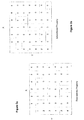
- FIGS 3a - 3d provide an informal description of the convex, concave, functional, min-closed, and max-closed properties.
- Each figure shows a matrix representation for the case of binary constraints (recalling, from Figure 1, that a binary constraint has two variables, here X and Y).
- Figure 3a shows a matrix representation of a row-convex property (or x-convex), which is characterised by the following pattern: if there are any 1's in a row (i.e. if, for a given value of the Y variable, there is more than one value in the domain of the X variable), then they will be grouped together. This can be seen from Figure 3a, where, for each row on which more than a single 1 appears, there are no gaps between the occurrences of the 1s.
- convex-related properties include a column-convex property (or y-convex), where in every column, the 1s, if any, are grouped together. From the column and row convex description it is easily deduced that a convex constraint is characterised by having, in every row and every column, the 1s, grouped together. Thus the matrix shown in Figure 3a is representative of a constraint that is row-convex, but which is not column-convex and thus not convex per-se.
- Figure 3b shows a constraint having x-functional property, which is characterised by having at most a single 1 per row.
- a constraint having y-functional property (not shown) can be characterised by having at most a single 1 per column
- a constraint having functional property per-se (not shown)
- the matrix shown in Figure 3b is representative of a constraint that is x-functional, but which is not y-functional and thus not functional per-se.
- Figure 3c shows a constraint having max-closed property, which is essentially an inference property, and infers information from existing values, namely that a constraint c, having solutions (u, v) and (u', v') also has a value at max(u, u') and max(v, v').
- a constraint c having solutions (u, v) and (u', v') also has a value at max(u, u') and max(v, v').
- Figure 3d shows a constraint having min-closed property, which is also an inference property, and infers information from existing values.
- a constraint is known to be either, or both, min-closed or/and max-closed, and only some of the values have been determined, then values can be inferred from existing values.
- a constraint, for which all values have been determined can be analysed (using the values) to determine whether or not it has the property of being min/max-closed.
- FIG. 4a is a schematic block diagram showing an arrangement in which embodiments of the invention may operate. Such an arrangement may be used for a scheduling problem, in particular for scheduling the allocation of jobs to a workforce.
- the arrangement comprises a database 01, which receives input specifications detailing, e.g., jobs to be processed, changes to resources (e.g. technician T1 is off sick) and conditions to be satisfied (e.g. job 1 has to be completed before job 2 etc.).
- the database 01 is in operative association with a constraint processing engine 03, hereinafter referred to as COL.
- COL constraint processing engine 03
- Innovative features of the invention include aspects of the COL 03 and are described in more detail below. However, in overview, the COL 03 extracts information from the database 01, constructs constraints based on the extracted information, and applies a variety of methods in an attempt to satisfy the constructed constraints.
- the COL 03 is also in operative association with a plurality of clients 05, 07, 09.
- a first of the clients is a scheduler 05, which receives problem variables, e.g. job and resource information, from the COL 03, together with problem expressions-e.g. problem constraints and optimisation function.
- the scheduler 05 attempts to optimise the optimisation function by applying changes to the variables and reviewing the performance of the optimisation function, until the performance satisfies a predetermined performance criterion.
- scheduler 05 makes changes to the variables, these changes have to be checked by the COL 03, to determine whether or not the changes violate, or satisfy, the constructed constraints.
- a second client is a repair client 07, which also receives problem variables and problem expressions of the kind described above from the COL 03.
- the problem variables and expressions are immediately input to the repair tool, which interacts with the COL 03 in an attempt to identify a valid solution for the modified values. Once a valid solution has been identified, it can be passed to the scheduler 05 for optimisation thereof.
- a third client is a user interaction client 09, which allows a user to effect direct changes to the problem variables and/or expressions, by, for example, removing a task. Any changes made in this manner are essentially equivalent to a change input to the database 01 as described above, and typically involves subsequent operation of the repair tool 07 and scheduler 05.
- the clients 05, 07, 09 could all be located on the same terminal, could each be located on a different terminal, and connected to the COL 03 via a Local Area Network (LAN) or similar means, or could each be located on a different terminal within separate networks.
- the database 01 could be located local to, or remote from, the COL 03 and the clients 05, 07, 09.
- Figure 4b shows a terminal T1 comprising a central processing unit (CPU) 401, a memory unit 403, an input/output device 405 for connecting the terminal T1 to the clients 05, 07, 09 and to the database 01; storage 407, and a suite of operating system programs 409, which control and co-ordinate low level operation of the terminal T1.
- CPU central processing unit
- memory unit 403 for storing data
- input/output device 405 for connecting the terminal T1 to the clients 05, 07, 09 and to the database 01
- storage 407 for controlling the terminal T1
- suite of operating system programs 409 which control and co-ordinate low level operation of the terminal T1.
- an inferencing engine 400 Generally embodiments of the invention are referred to as an inferencing engine 400, and comprise at least some of programs 411, 413, 415, 417. These programs, which are described in more detail below, are stored on storage 407 and are processable, under general control of the COL 03, by the CPU 401.
- the inferencing engine 400 also includes a constraint library LB, which stores constraints and properties relating thereto. It is understood that each of the programs 411, 413, 415, 417 could comprise a suite a of computer programs, and could be written in either, or a mixture, of the well known procedural or object-oriented programming paradigms.
- Embodiments of the invention are concerned with improving the domain reduction process described above, so that, in terms of the system presented in Figure 4a, the validity of changes made to variables - e.g. by the scheduler 05, or by the user interactive client 09, can be evaluated as efficiently as possible.
- Embodiments make use of the realisation that a constraint can be defined as a combination of other constraints. This then opens up the possibility for re-use of existing constraints, which have already been analysed for their properties, and have specific propagation mechanisms, which have been optimised according to properties, associated therewith. Thus, when a new constraint, for which a specific propagation mechanism does not exist, is received by the inferencing engine 400, the new constraint is expressed in terms of constraints already defined and accessible to the inferencing engine 400.
- New properties can be computed by defining operations, such as complementation (- P ), intersection ( ⁇ P ) and union ( ⁇ P ) (many more are possible), on properties.
- a problem with combining properties is that you have to close a set of (primitive) properties by intersection (i.e. compute all possible combinations-see example a few lines down) just to make sure that, for any constraint you want to specify, the strongest property for this constraint does indeed exist.
- A, B, C, D whose closure by set-intersection has 15 different members: A, B, C, D, A+B, A+C, A+D, B+C, B+D, C+D, A+B+C, A+B+D, A+C+D, B+C+D, A+B+C+D.
- the strongest property would be A+B+C+D.
- Embodiments of the present invention are thus focussed on deriving property information relating to new constraints, and are specifically concerned with re casting the properties into a format that allows them to be combined in a scalable manner, from which properties of the new constraint c 3 can be inferred.
- This format is based on a specific representation of constraint properties, referred to herein after as types, and on combining types in accordance with specific type operations.
- a type comprises a set of one or more primitive properties, and, once defined, can be utilised as a parameter of the constraint network.
- S p ⁇ fct, n, m ⁇ , where S p indicates a set of properties p, which, in this example includes functional (fct), reflexive (n), max-closed (m);
- the inferencing engine 400 also needs to know relationships between primitive properties, in particular to determine "stronger-than” relationships between primitive properties.
- a relationship between types can be expressed using a graph representation such as that presented in Figure 5.
- Figure 5 shows "stronger-than" relationships for unary constraint primitive properties: as a type is a subset of properties, each node in graph 500 represents a primitive property.
- the graph 500 shows that property convex 503 is weaker than the universal property 515, and property monotonic 507 is stronger than properties convex 503 and concave 505.
- Such a representation could be created manually, or automatically, based on previously defined ordering rules.
- This feature can be exploited to identify the properties associated with a type, which, in turn, can be used to identify an optimised propagation algorithm, as described in more detail in the context of the second example described below.
- Type operations provide an algebraic framework within which types can be combined in accordance with the constraint specification.
- c 3 c 1 ⁇ c 2
- SR() and SI() denote “stable by restriction” and “stable by intersection”, respectively.
- These stability expressions can be used to characterise a property.
- ⁇ T expressions involving different stability expressions, so-called stable by extension and stability by union, are used. The meaning of these stability expressions can be illustrated with reference to the matrix representation in Figure 3a.
- intersection of a convex constraint with another convex constraint will result in a 1 if and only if the two constraints individually have a 1 in that cell. It turns out that after intersection of convex constraints, the 1s (if any) in a row are continuous, meaning that the intersection operation on two convex constraints is convex, and the property convex is said to be "stable by intersection”.
- a property is stable by restriction if the intersection of any constraint satisfying the property with any other constraint is a constraint satisfying that property.
- a property is stable by extension if the union of any constraint satisfying the property with any other constraint is a constraint satisfying that property.
- t 3 is evaluated by performing a process referred to herein as "normalisation". Syntactically, the normalisation process is indicated by the presence of square brackets: [..], as can be seen from equation 1.
- Normalisation includes reviewing the ordering between the primitive properties in S p shown in Figure 5, and identifying all properties that include, and are weaker-than, type given by t 1 ⁇ T t 2 .
- the properties that are included in type functional can be identified: for this example, the properties are functional, convex and standard ( ⁇ fct ⁇ ⁇ ⁇ fct, cc x , std ⁇ ). These are the properties that are involved in new constraint c 3 , and these can be utilised to identify a propagation algorithm that is optimal for that constraint.
- Advantages of the embodiments include re-usability of existing constraint definitions and propagation algorithms, identification of an optimal propagation algorithm for a new constraint, usability (as, in the extreme case, the user merely has to specify the new constraint, and does not have to be an expert to use the system), scalable system that can handle complex constraint definitions comprising unary, binary, ternary etc. constraints.
- the feature of automatic identification of a bespoke propagation algorithm is entirely new.
- the components of the inferencing engine 400 include a program 411 for receiving a new constraint specification, which specification specifies a combination of constraints already stored, and defined, in COL 03.
- a user would input such a constraint specification to the receiving program 411.
- the components also include a program 413 for identifying constraint-type information from the library LB relating to the new constraint specification, and a program 415 for combining the identified constraint-type information in order to determine a type for the newly received constraint.
- program 415 derives properties associated with the determined type.
- the embodiment can also include a program 417 for creating a propagation method on the basis of the derived property and/or type.
- the constraint library LB mentioned above essentially comprises algebraic expressions involving one or more variables, each of which is an algebraic description of a constraint, and built-in operators that are able to interpret these algebraic expressions of the constraint.
- the library LB additionally stores type and property information, and a link to propagation methods relating to properties and types.
- the receiving program 411 receives 601 the new constraint specification, whereupon it passes 603 the specification to the identifying program 413.
- the identifying program 413 first detects 605 that there are 2 constraint operations,-(complement) and ⁇ (intersection), and that these are "nested" within one another.
- step 615 involves evaluating the following for the type operation ⁇ T :
- the combining program 415 then passes 619 these properties to the creating program 417, which uses 621 these properties to select an optimal propagation algorithm.
- this "use” involves the creating program 417 accessing 623 the library LB and comparing 625 the properties of the new constraint with properties stored therein (e.g. in an index to propagation algorithms) so as to identify suitable algorithms. Having identified one or more such algorithms from the index, the creating program 417 retrieves 627 the identified propagation algorithm(s) and assigns 629 the retrieved propagation algorithm to the new constraint.
- the creating program 417 will use the type to select an optimal propagation algorithm.
- the receiving program 411 receives 601 the constraint specification, whereupon it passes 603 the specification to the identifying program 413.
- the identifying program 413 first detects 605 that there are 2 constraint operations,-(complement) and ⁇ (union), and that these are "nested" within one another.
- Step 617 includes normalising the types, within the first and second nestings. Referring to Figure 5, for the present example, normalising the second, or outer, nesting [ ⁇ antif,std ⁇ gives ⁇ antif,concave,std ⁇ .
- This example illustrates the powerful inferencing ability of the embodiment: several equivalent sets of primitive properties for the new constraint can be identified, which enables selection of more than one optimal propagation algorithms for propagating the constraint.
- a third example, comprising constraint specification c -(c 1 (x) ⁇ c 2 (x)) ⁇ c 3 (x), is now described, again with reference to Figure 6.
- c 1 (x) is x>0
- c 2 (x) is x ⁇ 10
- the receiving program 411 receives 601 the constraint specification, whereupon it passes 603 the specification to the identifying program 413.
- the identifying program 413 first detects 605 that there are 3 constraint operations, - (complement), ⁇ (intersection) and ⁇ (union), and that these are "nested" within one another.
- Step 617 includes normalising types within the nestings; in this example there are three nestings, so that normalisation occurs three times.
- normalising type [ ⁇ fct ⁇ ] gives properties ⁇ fct, cv x , std ⁇ .
- type operations can be nested within other type operations, and the inner-most operation is evaluated first in the manner shown in these examples. It will thus readily be appreciated by one skilled in the art that any constraint can be "built" from existing constraints using basic combining operations such as complementation, union and intersection.
- relational operations and their type counterpart could be described, and used, provided a definition thereof were provided (e.g. stored in the library LB).
- An example of another relational operator is taking the converse of a binary relation, described below.
- the motivation for relational operations is of course constraint expressions: if a new constraint expression utilises a particular constraint operator (e.g. some sort of combinatory operation), then a corresponding type operator is required if the type of this new constraint is to be inferred using the invention.
- Each of the afore-mentioned examples describes a combination of unary constraints, which relate to the same variable (x).
- an embodiment of the invention can also be used to combine constraints relating to more than one variable - e.g. for a Vehicle Routing Problem, where the goal is to assign a sequence of visits to each vehicle in a fleet, an embodiment can be used to express conditions such as: "If a task starts (s) before 12:00am then its duration (d) is less than one hour". In this case, a first constraint (s ⁇ 12:00) involves variable s and a second constraint (d ⁇ 1.0) involves d.
- each of the two unary constraints first has to be "promoted" into a binary constraint.
- both the new constraint and the two known constraints (c 1 and c 2 ) are all of the same binary scope.
- the embodiment can further include a promoting program 419 (not shown) for promoting each of the unary constraints to corresponding binary constraints.
- FIG. 7 shows part of the unary graph 500 shown in Figure 5, namely convex, concave, functional, antifunctional, and monotonic for binary constraints. It can be seen that, in addition to convex and functional properties considered for unary constraints, binary constraints include x-convex, y-convex, x-functional, y-functional properties. This is to be expected, because binary constraints, by definition, have two dimensions, referred to here as x and y.
- the properties corresponding to the promoted binary constraint have to be identified. These can be identified from a store of mappings between properties of a unary constraint and types of a binary constraint.
- the type information is stored in the library LB as a look-up table, such as that shown in Table 1. This look-up table is generally manually created and updated whenever newly identified properties are added to the COL 03.
- Promoting c 1 to a binary constraint involves promoting c 1 (s) ⁇ c 1 (s,d), and promoting c 2 to a binary constraint involves promoting c 2 (s) ⁇ c 2 (d,s).
- both constraints have to be expressed in an identical form (i.e. either as c 1 (s,d) and c 2 (s,d) or as c 1 (d,s) and c 2 (d,s)). Accordingly, in the present example, c 2 is converted from c 2 (d,s) to c 2 (s,d).
- a converse operation can be applied to c 2 (d,s).
- f row-convex
- the converse thereof is property column-convex.
- the converse operation on types is defined "identically" to the complementation operation: the converse of a type is the set-union of the converses of the primitive properties of the type.
- c 1 (s) is promoted to a binary constraint on c 1 (s,d).
- the promoting program 419 refers to the mapping table to identify binary types corresponding to each of convex:un, concave:un, monotonic:un, standard:un, and retrieves the following types:
- c 2 (d) this is first promoted to c 2 (d,s), then, as c 1 and c 2 have to be expressed in the same format, c 2 (d,s) is transformed to c 2 (s,d), which involves applying a converse operation on type for c 2 (d,s).
- c 2 (s) is of the same type of c 1 (d), so that the type of c 2 (d,s) is also [monotonic:bin].
- Applying the converse operation on type [monotonic:bin] generates type [monotonic:bin], because the converse of monotonic is monotonic (referring to Figure 7 it can be seen that monotonic is stable by converse operation).
- constraint c 1 (s,d) has type [monotonic:bin] and constraint c 2 (s,d) has type [monotonic:bin].
- the identifying program 413 first searches for promoted binary constraints c 1 (s,d) and c 2 (s,d), together with the type information relating thereto. If such information is available, the identifying program 413 retrieves it. If, however, no such binary constraints exist, the promoting program 419 creates them, as described above, and sends the created binary constraints and type information directly to the identifying program 413 (in addition to storing in the library LB), which performs some or all of steps 601 - 629 described above.
- constraint c 3 could only be evaluated if user explicitly entered c 1 and c 2 as binary constraints.
- mappings such as the one described above is not limited to generating a binary constraint from unary constraints, but can be applied to generating a k-ary constraint. However, it is a prerequisite that the inferencing engine 400 has a mapping, such as that shown in Table 1, defining transformations between unary and k-ary properties.
- a constraint system such as that described above does not tell you anything about potential solutions to a problem, it merely evaluates whether values are consistent with the constraint network (where the constraint network is all of the constraints in a problem).
- the property information derived in accordance with embodiments of the invention could be used to identify information about solution viability and/or to modify constraint propagation process.
- the property and type information could be used to identify whether or not there is a solution to the problem.
- property information could be input to one or more expert rules that determine characteristics of a problem depending on network topology (constraints of problem) and property information. These expert rules could be stored in the Library LB, and applied in dependence on the property information, under control of another program (not shown).
- the property information could be used to select a relaxation method.
- the process of re-establishing consistency on a previously consistent network when one or several of its constraints are retracted is known as relaxation.
- relaxation The process of re-establishing consistency on a previously consistent network when one or several of its constraints are retracted.
- the whole problem i.e. all current constraints
- the whole problem has to be re-set (initial domains of variables are restored) and reevaluated (consistency has to be established from the beginning). This is expensive in terms of computing time, and it would be preferable to have a less expensive mechanism for relaxing a constraint network.
- Property information identified as described above could be used to develop a specialised (cheaper) relaxation method.
- the constraints used to build the new constraint c 3 are assumed to be available and accessible from the library LB.
- a user may want to define a new constraint and a corresponding new property corresponding thereto. The user would therefore have to specify the strength of this property with respect to the other properties (e.g. on a graph of properties, such as that shown in Figure 5), the complement property, and stability information relating to the property and the complement thereof (to enable the type algebra to be computed by the combining program), and make this information available, e.g. by storing it in the library LB.
Landscapes
- Engineering & Computer Science (AREA)
- Theoretical Computer Science (AREA)
- Computing Systems (AREA)
- Data Mining & Analysis (AREA)
- Evolutionary Computation (AREA)
- Physics & Mathematics (AREA)
- Computational Linguistics (AREA)
- General Engineering & Computer Science (AREA)
- General Physics & Mathematics (AREA)
- Mathematical Physics (AREA)
- Software Systems (AREA)
- Artificial Intelligence (AREA)
- Management, Administration, Business Operations System, And Electronic Commerce (AREA)
Abstract
The invention is concerned with improving methods of identifying
domains of variables that satisfy one or more predetermined constraints.
In an embodiment, constraints are expressed as a combination of
existing constraints, which have constraint properties and specific
optimised propagation mechanisms associated with them. The invention
utilises constraint property information because propagation methods are
coupled with properties, so that selection of an efficient propagation
method is dependent on constraint properties.
In the invention the nature of the combination of constraints is
assessed, and equivalent property operations are identified. A problem
with combining properties is that you have to close a set of
properties by intersection (i.e. compute all possible combinations).
Thus in the invention, the properties are cast into a format that
allows them to be combined in a scalable manner, from which properties
of the new constraint can be inferred.
This format is based on a specific representation of constraint
properties, referred to in the description as types, and on
combining types in accordance with specific type operations.
Description
- The present invention relates to a constraint analysis apparatus and method, and is suitable particularly, but not exclusively, for use in resource allocation problems.
- Constraint programming is a programming technology for solving complex combinatorial problems, where data representing a problem are described by variables, and conditions between the variables are represented by constraints. Each variable has an associated domain, which is a set of its potentially feasible values.
- Constraint programming is essentially a means of reducing domains of variables to values that satisfy whichever constraints are specified for a problem. The main applications areas of constraint programming include planning, scheduling, timetabling, routing, transmitter placement, frequency allocation, and network configuration, among others.
- Constraints describe different relationships that must be met within a set of variables in order to solve a problem. A process known as "domain reduction" allows computation of one, several, the best, or all of the values that may be solutions to the problem, and involves searching through the domains, dynamically and efficiently reducing the domains, thereby effectively shrinking the size of the problem. For more information the reader is referred to "Program != Program: Constraint Programming and its Relationship to Mathematical Programming", available from the Institute for Operations Research and the Management Science (INFORMS) 901 Elkridge Landing Road, Suite 400, Linthicum, Maryland 21090 USA.
- An example of a typical constraint based resource allocation problem is a vehicle routing problem, where the goal is to assign a sequence of jobs, or visits, to each vehicle in a fleet. A representation of variables and constraints comprising such a vehicle routing problem is shown in Figure 1, where variables si, di, ei, respectively represent the start time, duration and end time of a job ti. In the description, the terms "variable" and "domain variable" are used interchangeably. The constraints 100, 101, 102 in Figure 1 represent the following conditions: firstly the scheduling of jobs may have time constraints - e.g. a shop to which a delivery has to be made by one of the vehicles is open between 10 am and 12 pm; this can be represented by a unary constraint (100) 10:00 < si < 12:00. Secondly the end time for each job is given by the start time plus duration of the job; this can be represented by a ternary constraint (102) si+di = ei. Thirdly there are sequencing constraints, such as travel times (denoted as a constant, c), placed on job scheduling; this can be represented by a binary constraint (101) ei+c = sj, where sj is the start time of the next job (identified by j).
- A value, or a set of values, which satisfy the specified constraints, can be identified by carrying out the domain reduction process mentioned above. This method is generally referred to as a "propagation", or "filtering", method. Essentially, a propagation method systematically removes values, from the domains of the problem variables, which violate any of the problem constraints. For further information relating to these particular methods, the reader is referred to Mackworth, A.K. Consistency in Networks of Relations. Artificial Intelligence, Vol. 8(1), pp. 99-118, 1977.
- In order to focus on the specific contribution of the present invention, it is useful to first examine the methodology employed in the most general of these methods - a so-called "AC3" method. The strength of the AC3 method is that it can be applied to any sort of constraint; however, such comprehensive applicability incurs an efficiency cost: for a particular constraint, such a method typically involves many unnecessary computations. The methodology of the AC3 method is most easily illustrated by means of a simple example.
- Consider a problem that has two variables and two constraints, where the variables are x and t and the constraints are t>0 (C1) and x=t (C2). Each of the variables has a domain - i.e. a set of values; in this example, the domain of x is [0, 1, 2], the domain of t is [0, 1]. Referring to Figures 2a and 2b, the AC3 propagation method broadly comprises the following steps
- Step S 2.1 Pre-enforcement: look at each of the constraints, and remove all values from the domains that are incompatible with the constraints. List each variable that has had a change made to its domain.
- Step S 2.2 Place the, or each, changed variable in a stack 201 (a stack is alternatively referred to as a "queue" in the following description)
- Step S 2.3 Take the first variable 203 in the stack 201, and apply whichever constraint(s) include that first variable 203. The first variable 203 is x, and is included constraint in C2, so constraint C2 is applied to variables x and t. If, having applied the constraint to the variables, any of the variables have changed, place the changed variable on the bottom of the stack 201. Remove the first variable 203 from the stack.
- Step S 2.4 Take the next variable 205 in the stack 201, and apply whichever constraint(s) include that variable 205. The next variable 205 is t, and is included in constraints C1 and C2, so constraints C1, C2 are applied to variables x and t. If, having applied the constraint to the variables, any of the variables have changed, place the changed variable on the bottom of the stack 201. Remove the next variable 203 from the stack.
- Step S 2.5 Take the next variable 207 in the stack, and apply whichever constraint(s) include that variable 205. Variable x is the next variable 207, and is included constraint in C2, so constraint C2 is applied to variables x and t. If, having applied the constraint to the variables, any of the variables have changed, place the changed variable on the bottom of the stack 201. Remove the next variable 207 from the stack.
- As the stack is empty, the domains of variables x and t have been successfully reduced - namely x = [1], t = [1]. Clearly, if there had been more constraints, and if the variables x, t had had larger domains, the number of steps would increase accordingly.
- As can be seen, a problem with this method is that many redundant constraint checks can be carried out - essentially, and as illustrated by the example given in Figure 2a - the same pair of values may unnecessarily be checked many times in the course of reducing the domains of variables.
- Other propagation methods have been developed, each of which attempts to improve the efficiency in constraint checking by exploiting value-orientated propagation. The most efficient known propagation method is AC6, which records all values that satisfy a constraint as soon as they are discovered. This can be explained by means of an example: Consider a value u in the domain of x and a value v in the domain of y such that the pair (u,v) satisfies constraint c. In addition, assume there is no u' in x and v' in y such that c(u',v) and c(u,v'). In other words, u is the only compatible value for v and vice-versa. Assume constraint c is x=y. With the AC3 method, the pair (u,v) is systematically (and repeatedly) checked against c as described above with reference to Figure 2a, with the arguments u and v. With the AC6 method, as soon as this "positive hit" is encountered, it is recorded once and for all, and removed from the domain of values of x and y, thus avoiding future checks on these values.
- A user typically defines the constraints comprising his problem. With known systems, the user can define the constraints in one of the following ways:
- (1) Through an algebraic expression of variables, which is interpreted by built-in operators of the system. For instance, the user writes "x<y" and the system can automatically create a constraint c (<x,y>,"<") [meaning constraint c, involving 2 variables (x and y), wherein the relationship between them is <];
- (2) By constructing an object of a built-in generic functional or predicative constraint class having user-specified scope and user-specified function or predicate. For instance, the user can invoke a constructor of the predicative constraint class with the scope <x,y> and a binary predicate "bool test(u,v)" as arguments and the system will create a constraint c (<x,y>,test).
- (3) By defining a new kind of constraint - e.g. a new class that implements a specific predicate and some or all the propagation algorithms required (bound-/domain- consistency pre-filtering/filtering) and by constructing objects of this class with a scope.
-
- Method (1) guarantees optimal propagation for the constraints, since, to date, the best propagation algorithms are encoded for each kind of constraint (ie: method of propagating constraints have been tailored to suit the kind of constraint). However, its scope is limited to built-in constraints.
- Method (2) is the default constraint creation method and is particularly suited to non-expert users. It has the broadest scope since any constraint may be defined in this way, and it does not require any algorithm programming. However, it offers no performance guarantees since propagation relies on generic algorithms (i.e. constraints are propagated using either the AC3 or AC6 methods described above).
- Method (3) requires a clear understanding of propagation algorithms and good programming skills. For this reason, it is generally only used by expert users.
- As stated above, domain reduction simplifies computation of one, several, the best, or all of the solutions to the problem. A factor that determines how vigorously a domain is pruned is the scope of propagation applied to the domains. The scope of propagation essentially defines the extent to which the constraints must be satisfied within the domain of values making up the variable.
- The example described above employs so-called "domain consistency" scope (commonly referred to as "arc consistency"), where all of the values in the domains are checked against the constraints. An alternative to domain consistency is "bound consistency" scope, where just the bounds (ie. the max and min values) are checked against the constraints. A further alternative is "value consistency" scope (commonly referred to as "constraint checking"), where constraints are checked as soon as all of the variables involved therein are assigned a domain comprising a single value.
- As can be seen from the above paragraphs, a constraint essentially describes a relationship between variables. As is known in the art, constraints can be characterised by the logic properties of their relations, e.g. reflexivity, convexity, over a computation domain. A constraint property over Dk is any subset of k-ary relations over D, where D is the computation domain and k is the arity, or the number of variables in a constraint (e.g. referring back to Figure 1, constraint x =t has arity of 2 (binary constraint)).
- Examples of constraint properties include convexity, concavity, functionality, min-closedness, and max-closedness; each of these is essentially a mathematical description of characteristics of a constraint (so that, e.g. an inequality constraint, such as x<y, has certain characteristics that can be classified into a set of properties). In the following description, the term "primitive property" is interchangeably used with "property" per-se.
- As an alternative to a mathematical description of a property (which is set out in Appendix 1), properties can be illustrated via a matrix representation. This has the benefit of removing the mathematical complexity and thus allows us to explain the effect, or the significance, of a constraint in terms that are more easily understood by non-mathematical readers.
- Thus Figures 3a - 3d provide an informal description of the convex, concave, functional, min-closed, and max-closed properties. Each figure shows a matrix representation for the case of binary constraints (recalling, from Figure 1, that a binary constraint has two variables, here X and Y). The top-side and left-hand side of the matrix represent values in a domain (here [1...6] for each variable) and a 1 within the matrix indicates that the constraint is satisfied by the pair of values represented by that location. For example, if there is a 1 in location (1, 3) in the matrix, this indicates that the constraint is satisfied by the values X=1, Y=3, so that the domain includes values X = 1, Y = 3.
- Referring firstly to Figure 3a, this shows a matrix representation of a row-convex property (or x-convex), which is characterised by the following pattern: if there are any 1's in a row (i.e. if, for a given value of the Y variable, there is more than one value in the domain of the X variable), then they will be grouped together. This can be seen from Figure 3a, where, for each row on which more than a single 1 appears, there are no gaps between the occurrences of the 1s.
- Other convex-related properties (not shown) include a column-convex property (or y-convex), where in every column, the 1s, if any, are grouped together. From the column and row convex description it is easily deduced that a convex constraint is characterised by having, in every row and every column, the 1s, grouped together. Thus the matrix shown in Figure 3a is representative of a constraint that is row-convex, but which is not column-convex and thus not convex per-se.
- Figure 3b shows a constraint having x-functional property, which is characterised by having at most a single 1 per row. Conversely, a constraint having y-functional property (not shown) can be characterised by having at most a single 1 per column, while a constraint having functional property per-se (not shown), can be characterised by having at most a single 1 both per column and per row. Thus the matrix shown in Figure 3b is representative of a constraint that is x-functional, but which is not y-functional and thus not functional per-se.
- Figure 3c shows a constraint having max-closed property, which is essentially an inference property, and infers information from existing values, namely that a constraint c, having solutions (u, v) and (u', v') also has a value at max(u, u') and max(v, v'). For example, referring to cell location (3, 1) and cell location (2, 2), it can be seen that there are 1s in each cell. Taking the maximum of these two co-ordinates, X=3 and Y=2, then there will also be a 1 at (3, 2).
- Figure 3d shows a constraint having min-closed property, which is also an inference property, and infers information from existing values. In this case, it can be inferred that a constraint c, having values (u, v) and (u', v') also has a value at min(u, u') and min(v, v'). For example, referring to cell location (3, 1) and cell location (2, 2), it can be seen that there are 1s in each cell. Taking the minimum of these two co-ordinates, X = 2 and Y = 1, then there will also be a 1 at (2, 1).
- Thus, if a constraint is known to be either, or both, min-closed or/and max-closed, and only some of the values have been determined, then values can be inferred from existing values. Alternatively, a constraint, for which all values have been determined, can be analysed (using the values) to determine whether or not it has the property of being min/max-closed.
- There is a group of properties: row-concave, column-concave, and concave per se (not shown), and each of these is the reverse (or converse) of its convex property counter-part, so that, for example, a constraint having a row-concave property has 0s grouped together on a row.
- Other terms that are commonly used when discussing a constraint system, and which are used in the following description, include completeness, strongest property and constraint network. These are defined as follows:
- "completeness": a measure of the efficiency of a system, and indicates the ability of the system to identify the strongest property, where the "strongest property" is the set intersection (or logical conjunction) of all properties that a constraint satisfies. Evaluating the "soundness" and "completeness" of a system is a generally accepted way of evaluating any inference system.
- "constraint network": all of the constraints in a problem.
-
- For ease of reference for the reader, the definitions of these, and other terms discussed above and below, are provided in Appendix A.
- According to the present invention, there is provided a method or system as set out in the accompanying claims. Further aspects of the invention will be apparent from the following description of preferred embodiments of the invention, which are given by way of example only and with reference to the accompanying drawings, in which
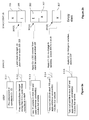
- Figure 1 is a schematic representation of conventional n-ary constraints;
- Figure 2a is a flow diagram showing steps involved in conventional constraint propagation methods;
- Figure 2b is a schematic representation of the organisation of variables in conventional constraint propagation methods;
- Figure 3a is a schematic representation of the property row-convexity;
- Figure 3b is a schematic representation of the property x-functionality;
- Figure 3c is a schematic representation of the property max-closedness;
- Figure 3d is a schematic representation of the property min-closedness;
- Figure 4a is a schematic representation of operating environment of embodiments of the invention;
- Figure 4b is a schematic representation of an embodiment of the invention;
- Figure 5 is a schematic representation of unary inter-property relationships, as utilised by embodiments of the invention;
- Figure 6 is a block diagram showing operation of a first embodiment of the invention; and
- Figure 7 is a schematic representation of binary inter-property relationships, as utilised by embodiments of the invention.
-
- Figure 4a is a schematic block diagram showing an arrangement in which embodiments of the invention may operate. Such an arrangement may be used for a scheduling problem, in particular for scheduling the allocation of jobs to a workforce. The arrangement comprises a database 01, which receives input specifications detailing, e.g., jobs to be processed, changes to resources (e.g. technician T1 is off sick) and conditions to be satisfied (e.g. job 1 has to be completed before job 2 etc.). The database 01 is in operative association with a constraint processing engine 03, hereinafter referred to as COL. Innovative features of the invention include aspects of the COL 03 and are described in more detail below. However, in overview, the COL 03 extracts information from the database 01, constructs constraints based on the extracted information, and applies a variety of methods in an attempt to satisfy the constructed constraints.
- The COL 03 is also in operative association with a plurality of clients 05, 07, 09. A first of the clients is a scheduler 05, which receives problem variables, e.g. job and resource information, from the COL 03, together with problem expressions-e.g. problem constraints and optimisation function. The scheduler 05 attempts to optimise the optimisation function by applying changes to the variables and reviewing the performance of the optimisation function, until the performance satisfies a predetermined performance criterion.
- If the scheduler 05 makes changes to the variables, these changes have to be checked by the COL 03, to determine whether or not the changes violate, or satisfy, the constructed constraints. The process of attempting to optimise a solution (by the scheduler 05), then checking that the said solution satisfies the constraints (by the COL 03), is typically an iterative process.
- A second client is a repair client 07, which also receives problem variables and problem expressions of the kind described above from the COL 03. In overview, when a change is input to the database 01, which is likely to render a currently valid solution invalid, the problem variables and expressions are immediately input to the repair tool, which interacts with the COL 03 in an attempt to identify a valid solution for the modified values. Once a valid solution has been identified, it can be passed to the scheduler 05 for optimisation thereof.
- A third client is a user interaction client 09, which allows a user to effect direct changes to the problem variables and/or expressions, by, for example, removing a task. Any changes made in this manner are essentially equivalent to a change input to the database 01 as described above, and typically involves subsequent operation of the repair tool 07 and scheduler 05.
- The clients 05, 07, 09 could all be located on the same terminal, could each be located on a different terminal, and connected to the COL 03 via a Local Area Network (LAN) or similar means, or could each be located on a different terminal within separate networks. The database 01 could be located local to, or remote from, the COL 03 and the clients 05, 07, 09.
- Features of the constraint processing engine COL 03 are now described, with reference to Figures 4a, 4b, 5 and 6.
- Figure 4b shows a terminal T1 comprising a central processing unit (CPU) 401, a memory unit 403, an input/output device 405 for connecting the terminal T1 to the clients 05, 07, 09 and to the database 01; storage 407, and a suite of operating system programs 409, which control and co-ordinate low level operation of the terminal T1.
- Generally embodiments of the invention are referred to as an inferencing engine 400, and comprise at least some of programs 411, 413, 415, 417. These programs, which are described in more detail below, are stored on storage 407 and are processable, under general control of the COL 03, by the CPU 401. The inferencing engine 400 also includes a constraint library LB, which stores constraints and properties relating thereto. It is understood that each of the programs 411, 413, 415, 417 could comprise a suite a of computer programs, and could be written in either, or a mixture, of the well known procedural or object-oriented programming paradigms.
- Embodiments of the invention are concerned with improving the domain reduction process described above, so that, in terms of the system presented in Figure 4a, the validity of changes made to variables - e.g. by the scheduler 05, or by the user interactive client 09, can be evaluated as efficiently as possible.
- Embodiments make use of the realisation that a constraint can be defined as a combination of other constraints. This then opens up the possibility for re-use of existing constraints, which have already been analysed for their properties, and have specific propagation mechanisms, which have been optimised according to properties, associated therewith. Thus, when a new constraint, for which a specific propagation mechanism does not exist, is received by the inferencing engine 400, the new constraint is expressed in terms of constraints already defined and accessible to the inferencing engine 400.
- Consider an example of a new constraint c3, which can be defined as c3=c1 ∩c2 (where c1 and c2 are known). Having realised that a new constraint can be expressed as a combination of other, previously defined and optimised constraints, another realisation is that the property information relating to constraints c1 and c2 can be exploited in order to determine a property for c3.
- New properties can be computed by defining operations, such as complementation (-P), intersection (∩P) and union (∪P) (many more are possible), on properties. However, a problem with combining properties is that you have to close a set of (primitive) properties by intersection (i.e. compute all possible combinations-see example a few lines down) just to make sure that, for any constraint you want to specify, the strongest property for this constraint does indeed exist. Consider a set of four properties A, B, C, D whose closure by set-intersection has 15 different members: A, B, C, D, A+B, A+C, A+D, B+C, B+D, C+D, A+B+C, A+B+D, A+C+D, B+C+D, A+B+C+D. In this example, the strongest property would be A+B+C+D.
- The property operation(s) involved in a new constraint, say, c3=c1 ∩ c2 is ∩p, and this would have to be defined for each member of the set. For example, the set of properties (where a property is denoted as pi) for p3 = p1 ∩p p2 will involve a 15x15 matrix, where each element of the matrix has been specified for property intersection between members of the set; if c3 involved a mixture of, say union, intersection and complementation of c1 and c2 and other constraints, the property algebra would additionally involve at least a 15x15 matrix for union and a vector of size 15 for complementation of properties.
- The major motivation for identifying properties associated with constraints is that propagation methods and consistency scopes are coupled with properties, so that selection of an efficient propagation method and scope of consistency is dependent on constraint properties. For example, if a constraint can be identified as being monotonic, then only the maximum and minimum values of the domains need to be checked (for monotonic constraints, such as x<y, enforcing bound-consistency is equivalent to enforcing domain-consistency, because the result is the same for both domain and bound consistency). As a result the domain can be reduced using bound consistency. In the absence of any knowledge of constraint properties, the constraint would have to be evaluated over the whole domain (i.e. applying arc, (domain) consistency), which incurs unnecessary overheads in terms of processing.
- Thus knowledge about constraint properties enables selection of optimum propagation algorithms, which results in faster domain reduction and faster validation of potential solutions.
- Embodiments of the present invention are thus focussed on deriving property information relating to new constraints, and are specifically concerned with recasting the properties into a format that allows them to be combined in a scalable manner, from which properties of the new constraint c3 can be inferred.
- This format is based on a specific representation of constraint properties, referred to herein after as types, and on combining types in accordance with specific type operations.
- A type comprises a set of one or more primitive properties, and, once defined, can be utilised as a parameter of the constraint network. e.g. for Sp = {fct, n, m}, where Sp indicates a set of properties p, which, in this example includes functional (fct), reflexive (n), max-closed (m);
- a type t1 = {fct, n} corresponds to the properties "functional and reflexive"
- a type t2 = {m} corresponds to the property "max-closed"
- The inferencing engine 400 also needs to know relationships between primitive properties, in particular to determine "stronger-than" relationships between primitive properties. A relationship between types can be expressed using a graph representation such as that presented in Figure 5. Figure 5 shows "stronger-than" relationships for unary constraint primitive properties: as a type is a subset of properties, each node in graph 500 represents a primitive property. The graph 500 shows that property convex 503 is weaker than the universal property 515, and property monotonic 507 is stronger than properties convex 503 and concave 505. Such a representation could be created manually, or automatically, based on previously defined ordering rules.
- Thus a "stronger-than" relationship between primitive properties, such as the graph representation shown in Figure 5 (including representations for binary, ternary etc. constraints), is defined, and accessible from the library LB.
- Inspection of Figure 5 shows that non-identical types may be equivalent (i.e. non-identical types may have identical intersection of properties)
- Type operations provide an algebraic framework within which types can be combined in accordance with the constraint specification. Thus for the example c3=c1 ∩ c2, the corresponding type definition is t3=t1 ∩T t2, which includes type operation ∩T . In a first embodiment, type operation ∩T involves so-called "stability expressions" SR(), Sl((), which are combined in a manner that is dependent on the nature of the combination between c1 and c2 (here intersection):
- In equation 1, SR() and SI() denote "stable by restriction" and "stable by intersection", respectively. These stability expressions can be used to characterise a property. For a union type operator, ∪T, expressions involving different stability expressions, so-called stable by extension and stability by union, are used. The meaning of these stability expressions can be illustrated with reference to the matrix representation in Figure 3a.
- Referring to the matrix shown in Figure 3a, for each cell therein, intersection of a convex constraint with another convex constraint will result in a 1 if and only if the two constraints individually have a 1 in that cell. It turns out that after intersection of convex constraints, the 1s (if any) in a row are continuous, meaning that the intersection operation on two convex constraints is convex, and the property convex is said to be "stable by intersection".
- Conversely, of each cell of the matrix, union of a convex constraint with another convex constraint will result in a 1 if either, or both, of the constraints have a 1 in the corresponding cell. It turns out that after union of convex constraints, the 1s (if any) in a row may be discontinuous, meaning that the union operation on two convex constraints is NOT convex in general, and the property convex is not said to be "stable by union".
- A property is stable by restriction if the intersection of any constraint satisfying the property with any other constraint is a constraint satisfying that property. A property is stable by extension if the union of any constraint satisfying the property with any other constraint is a constraint satisfying that property.
- These stability features, and other definitions of type combinations, are either stored in, or also accessible via, the library LB (formal definitions of SR, SI, SE, SU are defined in Appendix A of the description).
- Having evaluated the expression SR(t 1)∪SR(t 2)∪SI(t 1 ∩t 2), t3 is evaluated by performing a process referred to herein as "normalisation". Syntactically, the normalisation process is indicated by the presence of square brackets: [..], as can be seen from equation 1.
- Normalisation includes reviewing the ordering between the primitive properties in Sp shown in Figure 5, and identifying all properties that include, and are weaker-than, type given by t 1 ∩T t 2. For example, if, upon application of Equation 1, the type given by t 1 ∩T t 2 turned out to be type functional (fct), then with reference to Figure 5, the properties that are included in type functional can be identified: for this example, the properties are functional, convex and standard ({fct} ≡ {fct, ccx, std}). These are the properties that are involved in new constraint c3, and these can be utilised to identify a propagation algorithm that is optimal for that constraint.
- Advantages of the embodiments include re-usability of existing constraint definitions and propagation algorithms, identification of an optimal propagation algorithm for a new constraint, usability (as, in the extreme case, the user merely has to specify the new constraint, and does not have to be an expert to use the system), scalable system that can handle complex constraint definitions comprising unary, binary, ternary etc. constraints. The feature of automatic identification of a bespoke propagation algorithm is entirely new.
- The components of the inferencing engine 400, together with the operation thereof when deriving properties of a newly defined constraint, will now be described in more detail, with reference to Figures 4a - 8.
- Referring to Figure 4b, the components of the inferencing engine 400 include a program 411 for receiving a new constraint specification, which specification specifies a combination of constraints already stored, and defined, in COL 03. For example, if constraints c1 and c2 have already been entered to the COL 03, a new constraint specification could include, for example c3=c1 ∩c2. Typically a user would input such a constraint specification to the receiving program 411.
- The components also include a program 413 for identifying constraint-type information from the library LB relating to the new constraint specification, and a program 415 for combining the identified constraint-type information in order to determine a type for the newly received constraint. In addition program 415 derives properties associated with the determined type. The embodiment can also include a program 417 for creating a propagation method on the basis of the derived property and/or type.
- The constraint library LB mentioned above essentially comprises algebraic expressions involving one or more variables, each of which is an algebraic description of a constraint, and built-in operators that are able to interpret these algebraic expressions of the constraint. The library LB additionally stores type and property information, and a link to propagation methods relating to properties and types.
- Use of the inferencing engine 400 is now described, by means of several examples. The first example is shown in Figure 6, which is a flow diagram showing the steps involved in identifying a type associated with a new constraint c3(x) from known constraints c1(x) and c2(x):
and accesses 609 the library LB in order to extract type operations corresponding to the types, thereby retrieving 611 the following information: - t1 = {concave (ccv), antifunctional (antif), standard (std)}
- t2 = {convex (cvx), concave (ccv), monotonic (mon) , standard (std)} and the following type operations:
-
-
-
- SR(-T (t 1)) = {fct,std}
- SR(t 2) = {std}
- SI(-T (t 1)∩t 2) = SI({cvx }) = {cvx,std}
- -T (t 1)∩ T t 2 = [SR(- T (t 1))∪SR(t 2)∪SI(- T (t 1)∩t 2)]= [{fct}∪{cvx }] = [{fct},{cvx },{std}]
- The combining program 415 then passes 619 these properties to the creating program 417, which uses 621 these properties to select an optimal propagation algorithm. In a first instance, this "use" involves the creating program 417 accessing 623 the library LB and comparing 625 the properties of the new constraint with properties stored therein (e.g. in an index to propagation algorithms) so as to identify suitable algorithms. Having identified one or more such algorithms from the index, the creating program 417 retrieves 627 the identified propagation algorithm(s) and assigns 629 the retrieved propagation algorithm to the new constraint.
- As an alternative to steps 619 - 623, if the index is configured to store information in terms of types, either in addition to, or instead of, properties, the creating program 417 will use the type to select an optimal propagation algorithm.
- Note that the property "standard" (std) appears in all types, so it could be removed from the set of primitive properties.
- A second example, comprising constraint specification c3(x)=c1(x) ∪ -c2(x), is now described, also with reference to Figure 6. In this second example c1(x) is x ≠ 2 and c2(x) is x>0.
- The receiving program 411 receives 601 the constraint specification, whereupon it passes 603 the specification to the identifying program 413. The identifying program 413 first detects 605 that there are 2 constraint operations,-(complement) and ∪ (union), and that these are "nested" within one another. The identifying program 413 transposes 607 the constraint algebra into type algebra:
- t1 = {concave (ccv), antifunctional (antif), standard (std)}
- t2 = {convex (cvx), concave (ccv), monotonic (mon), standard (std)} and the following type operations:
- first nesting:
-T (t 2) = {ccv,cvx,mon,std} (the complement of monotonic is monotonic (refer Figure 5)) - second nesting:
- SE(t 1) = {std,antif}
- SE(-T (t 2)) = {std}
- SU(t 1)∩-T (t 2) = SU({ccv }) = {std,antif}
-
- As for the first example, Step 617 includes normalising the types, within the first and second nestings. Referring to Figure 5, for the present example, normalising the second, or outer, nesting [{antif,std} gives {antif,concave,std}.
- This example illustrates the powerful inferencing ability of the embodiment: several equivalent sets of primitive properties for the new constraint can be identified, which enables selection of more than one optimal propagation algorithms for propagating the constraint.
- A third example, comprising constraint specification c=-(c1(x) ∪ c2(x)) ∩ c3(x), is now described, again with reference to Figure 6. In this third example c1(x) is x>0, c2(x) is x ≠10 and c3(x) is x=5.
- As for the two previous examples, the receiving program 411 receives 601 the constraint specification, whereupon it passes 603 the specification to the identifying program 413. The identifying program 413 first detects 605 that there are 3 constraint operations, - (complement), ∩ (intersection) and ∪ (union), and that these are "nested" within one another. The identifying program 413 transposes 607 the constraint algebra into type algebra:
- t1 = { convex (cvx), concave (ccv), monotonic (mon)}
- t2 = { antifunctional (antif)}
- t3 = { functional (fct)} together with the following type operations:
- first nesting (t'):
- SE(t 1) = {std}
- SE(t 2) = {antif}
- SU(t 1)∩(t 2) = SU({ccv }) = {ccv}
- second nesting (t''):
- third nesting:
-
- As for the first and second examples, Step 617 includes normalising types within the nestings; in this example there are three nestings, so that normalisation occurs three times. Referring to Figure 5, for the third (outer) nesting, normalising type [{fct}] gives properties {fct, cvx, std}.
- This example illustrates the recursive nature of the type algebra: type operations can be nested within other type operations, and the inner-most operation is evaluated first in the manner shown in these examples. It will thus readily be appreciated by one skilled in the art that any constraint can be "built" from existing constraints using basic combining operations such as complementation, union and intersection.
- Although the examples described thus far are concerned with union, complementation and intersection, other relational operations and their type counterpart could be described, and used, provided a definition thereof were provided (e.g. stored in the library LB). An example of another relational operator is taking the converse of a binary relation, described below. The motivation for relational operations is of course constraint expressions: if a new constraint expression utilises a particular constraint operator (e.g. some sort of combinatory operation), then a corresponding type operator is required if the type of this new constraint is to be inferred using the invention.
- Each of the afore-mentioned examples describes a combination of unary constraints, which relate to the same variable (x). However, an embodiment of the invention can also be used to combine constraints relating to more than one variable - e.g. for a Vehicle Routing Problem, where the goal is to assign a sequence of visits to each vehicle in a fleet, an embodiment can be used to express conditions such as: "If a task starts (s) before 12:00am then its duration (d) is less than one hour". In this case, a first constraint (s<12:00) involves variable s and a second constraint (d<1.0) involves d.
- These two unary constraints are combined by a logical "If THEN" expression to output a binary constraint involving both s and d. Mathematically, this expression IF c1 THEN c2 is formulated in terms of negation (¬) and union (v) as ¬c1∨c2.
- Thus in addition to the steps described above with reference to Figure 6, if a new constraint involves creating a binary constraint from two unary constraints, each of the two unary constraints first has to be "promoted" into a binary constraint. In this way both the new constraint and the two known constraints (c1 and c2) are all of the same binary scope. Accordingly the embodiment can further include a promoting program 419 (not shown) for promoting each of the unary constraints to corresponding binary constraints.
- Promoting a constraint to a binary order affects the properties associated with the constraint because binary properties are different to unary properties. Figure 7 shows part of the unary graph 500 shown in Figure 5, namely convex, concave, functional, antifunctional, and monotonic for binary constraints. It can be seen that, in addition to convex and functional properties considered for unary constraints, binary constraints include x-convex, y-convex, x-functional, y-functional properties. This is to be expected, because binary constraints, by definition, have two dimensions, referred to here as x and y.
- Thus, in addition to promoting the unary constraint to a binary constraint, the properties corresponding to the promoted binary constraint have to be identified. These can be identified from a store of mappings between properties of a unary constraint and types of a binary constraint. Preferably the type information is stored in the library LB as a look-up table, such as that shown in Table 1. This look-up table is generally manually created and updated whenever newly identified properties are added to the COL 03.
Property for unary constraint over (x) Resulting type for binary constraint over (x,y) Properties corresponding to normalized type functional:un [convex:bin] standard, convex, x-convex, y-convex, y-functional antifunctional:un [concave:bin] standard, concave, x-concave, y-concave, y-antifunctional convex:un [convex :bin] standard, convex, x-convex, y-convex concave:un [concave:bin] standard, concave, x-concave, y-concave standard:un [standard:bin] standard monotonic:un [monotonic:bin] standard, monotonic, convex, x-convex, y-convex, concave, x-concave, y-concave - Recalling the current example, c1 = s<12:00 and c2 = d<1.0.
- Promoting c1 to a binary constraint involves promoting c1(s)→c1(s,d), and promoting c2 to a binary constraint involves promoting c2(s)→c2(d,s). When creating a new constraint c3 from a combination of c1 and c2, both constraints have to be expressed in an identical form (i.e. either as c1(s,d) and c2(s,d) or as c1(d,s) and c2(d,s)). Accordingly, in the present example, c2 is converted from c2(d,s) to c2(s,d).
- To effect this conversion (i.e. to obtain c2(s,d) from c2(d,s)), a converse operation can be applied to c2(d,s). Essentially, if the mapping f(x)→(x,y) is implemented, then the mapping g(x)→(y,x) can be obtained by applying the first mapping (f:(x)→(x,y)) and then applying the converse operation on the result of the first mapping. That is, g(c)=converse (f(c)). For example, if property A is row-convex, the converse thereof is property column-convex. The converse operation on types is defined "identically" to the complementation operation: the converse of a type is the set-union of the converses of the primitive properties of the type.
- Referring back to the example, c1(s) is promoted to a binary constraint on c1(s,d). c1(s) is of type monotonic, which involves [monotonic:un] = {convex:un, concave:un, monotonic:un, standard:un}. The promoting program 419 refers to the mapping table to identify binary types corresponding to each of convex:un, concave:un, monotonic:un, standard:un, and retrieves the following types:
- [convex:bin], [concave:bin], [std:bin] and [monotonic:bin]. Referring to Figure 7, it can be seen that
- type [convex:bin] ≡ {xconvex, yconvex, std}
- type [concave:bin] ≡ {xconcave, yconcave, std}
- type [std:bin] ≡ {std}
- type [monotonic:bin] ≡ {concave, xconcave, yconcave, convex, xconvex, yconvex, std} so that [monotonic:bin] encompasses all of the properties involved in c1 = c1(s,d), and is the type of promoted c1(s,d).
-
- Turning now to c2(d), this is first promoted to c2(d,s), then, as c1 and c2 have to be expressed in the same format, c2(d,s) is transformed to c2(s,d), which involves applying a converse operation on type for c2(d,s). c2(s) is of the same type of c1(d), so that the type of c2(d,s) is also [monotonic:bin]. Applying the converse operation on type [monotonic:bin] generates type [monotonic:bin], because the converse of monotonic is monotonic (referring to Figure 7 it can be seen that monotonic is stable by converse operation).
- Thus constraint c1(s,d) has type [monotonic:bin] and constraint c2(s,d) has type [monotonic:bin].
- Thus when receiving program 411 receives 601 constraint specification ¬c1∨c2 for constraints c1 = s < 12:00 and c2 = d < 1.0, the identifying program 413 first searches for promoted binary constraints c1(s,d) and c2(s,d), together with the type information relating thereto. If such information is available, the identifying program 413 retrieves it. If, however, no such binary constraints exist, the promoting program 419 creates them, as described above, and sends the created binary constraints and type information directly to the identifying program 413 (in addition to storing in the library LB), which performs some or all of steps 601 - 629 described above.
- If the type mappings and converse operator were not defined in the inferencing engine 400, constraint c3 could only be evaluated if user explicitly entered c1 and c2 as binary constraints.
- The skilled person will appreciate that a mapping such as the one described above is not limited to generating a binary constraint from unary constraints, but can be applied to generating a k-ary constraint. However, it is a prerequisite that the inferencing engine 400 has a mapping, such as that shown in Table 1, defining transformations between unary and k-ary properties.
- In general, a constraint system such as that described above does not tell you anything about potential solutions to a problem, it merely evaluates whether values are consistent with the constraint network (where the constraint network is all of the constraints in a problem).
- In addition to identifying propagation algorithms for a new constraint, the property information derived in accordance with embodiments of the invention could be used to identify information about solution viability and/or to modify constraint propagation process.
- Firstly, the property and type information could be used to identify whether or not there is a solution to the problem. For example, property information could be input to one or more expert rules that determine characteristics of a problem depending on network topology (constraints of problem) and property information. These expert rules could be stored in the Library LB, and applied in dependence on the property information, under control of another program (not shown).
- For example, if the combining program 415 has determined that all of the constraints of the problem are binary and min-max closed, then this could be input to the other program, which triggers processing of the following expert rule:
- "IF bound-consistency does not fail on this problem, THEN the resulting minimum values of the variables provide a solution to the problem". Thus the constraints could be propagated with a propagation algorithm that is optimised for bound-consistency, and, if the constraints are consistent, the inferencing engine 400 can deduce that there is a solution to the problem.
-
- Secondly the property information could be used to select a relaxation method. The process of re-establishing consistency on a previously consistent network when one or several of its constraints are retracted is known as relaxation. With existing systems, when a constraint is retracted, the whole problem (i.e. all current constraints) has to be re-set (initial domains of variables are restored) and reevaluated (consistency has to be established from the beginning). This is expensive in terms of computing time, and it would be preferable to have a less expensive mechanism for relaxing a constraint network.
- Property information identified as described above could be used to develop a specialised (cheaper) relaxation method. For example, when all constraints in the problem are of the same, or equivalent, type (as defined above), such as x = y, y = z, z = x, upon program definition, another program (not shown) could log the fact that the constraints have the same property, namely equality. If, once the constraint network has been propagated, constraint z = x were retracted from the problem, the other program could be consulted to determine the relationship between the constraints. If the constraints were equality constraints, this means that removal of one of the constraints has no effect on the network. In this example, the properties are indeed homogenous, so there is no need to re-evaluate the constraint network.
- In the embodiments described above, the constraints used to build the new constraint c3 are assumed to be available and accessible from the library LB. In some situations, a user may want to define a new constraint and a corresponding new property corresponding thereto. The user would therefore have to specify the strength of this property with respect to the other properties (e.g. on a graph of properties, such as that shown in Figure 5), the complement property, and stability information relating to the property and the complement thereof (to enable the type algebra to be computed by the combining program), and make this information available, e.g. by storing it in the library LB.
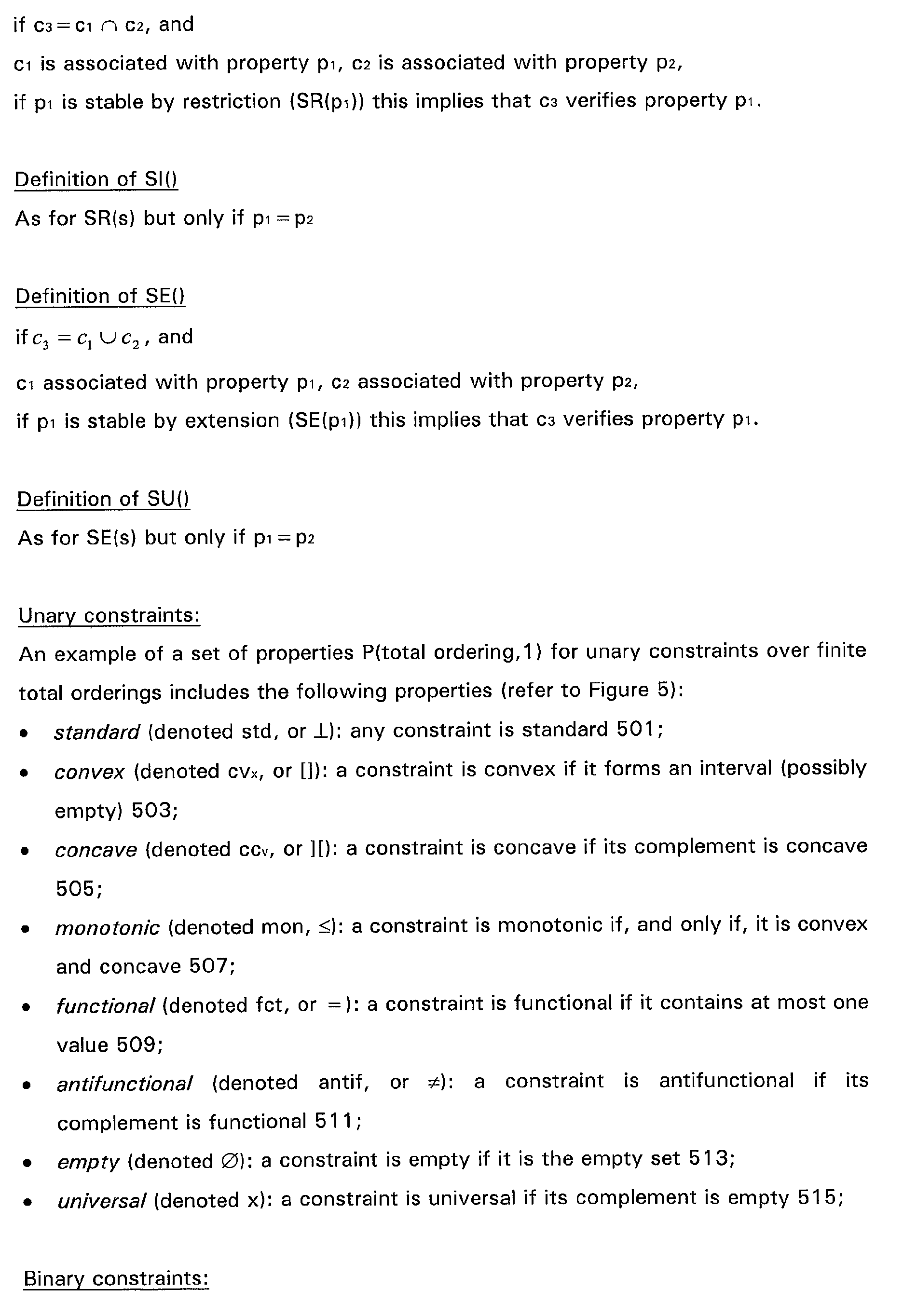


Claims (9)
- Apparatus for identifying a property associated with a constraint, a property being a characteristic of a constraint and being for use in identifying an algorithm for propagation of the constraint in a resource allocation problem, the apparatus comprising:(i) storage (LB) for storing
an ordering (500) between properties of constraints;
constraints and types associated with the constraints, wherein a type is a conjunction of properties;
a plurality of processable specifications (A1, A2, A3) for combining types in accordance with any of a plurality of combinatorial type operators;(ii) receiving means (411) for receiving a constraint, the received constraint being expressed as a combination of at least two stored constraints;(iii) retrieving means (413) for retrieving the at least two stored constraints involved in the received constraint;(iv) means (413) for
analysing the combination of the at least two constraints in order to identify a combinatorial type operator corresponding thereto, and
retrieving a specification associated with the identified combinatorial type operator;(v) processing means (415) for processing the retrieved specification, thereby identifying a type associated with the new constraint;(vi) accessing means (415) for accessing the ordering between properties stored in the store so as to identify one or more properties associated with the or each identified type. - Apparatus according to claim 1, wherein the storage (LB) further includes a mapping between properties and algorithms and the apparatus further includes means (417) for accessing the mappings stored in the store so as to identify an algorithm corresponding to the or each retrieved property.
- Apparatus according to claim 1 or claim 2, wherein, when the received constraint involves more than one kind of combination of the at least two constraints, the means (413) is arranged to analyse the relationship between the combinations and the processing means (415) is arranged to recursively process corresponding retrieved specifications in accordance with the analysed relationship.
- Apparatus according to any one of the preceding claims, wherein the means (413) is further arranged to identify variables involved in each of the at least two constraints, and, if one of the constraints involves a variable that is not involved in one or more of the other constraints, the means (413) is arranged to modify each of the said constraints so that each constraint involves the same variables.
- A method of identifying a property associated with a constraint, a property being a characteristic of a constraint and being for use in identifying an algorithm for a resource allocation problem, the method including the steps of:receiving (601) a constraint, the received constraint being expressed as a combination of at least two constraints;analysing (605) the combination of the at least two constraints in order to identify a combinatorial type operator corresponding thereto;retrieving (609) types associated with the at least two constraints, wherein a type is a conjunction of properties;retrieving (611) a specification for combining types associated with the identified combinatorial type operator;processing (615) the retrieved specification, thereby identifying one or more types associated with the new constraint;accessing (617) an ordering between properties so as to identify one or more properties associated with the or each identified type.
- A method according to claim 5, further including accessing (623) a mapping between properties and algorithms so as to identify (627) an algorithm corresponding to the or each retrieved property.
- A method according to claim 6, including applying the identified algorithm when propagating the received constraint during evaluation of a resource allocation problem that includes the received constraint.
- A method according to claim 6 or claim 7, further including the steps of identifying variables involved in each of the at least two constraints, and, if one of the constraints involves a variable that is not involved in one or more of the other constraints, modifying each of the said constraints so that each constraint involves the same variables.
- A method according to claim 8, wherein the modifying step includes reviewing the properties associated with each of the at least two unmodified constraints in order to determine corresponding properties for the modified constraints.
Priority Applications (1)
| Application Number | Priority Date | Filing Date | Title |
|---|---|---|---|
| EP01310038A EP1316916A1 (en) | 2001-11-30 | 2001-11-30 | Constraint analysis apparatus and method |
Applications Claiming Priority (1)
| Application Number | Priority Date | Filing Date | Title |
|---|---|---|---|
| EP01310038A EP1316916A1 (en) | 2001-11-30 | 2001-11-30 | Constraint analysis apparatus and method |
Publications (1)
| Publication Number | Publication Date |
|---|---|
| EP1316916A1 true EP1316916A1 (en) | 2003-06-04 |
Family
ID=8182499
Family Applications (1)
| Application Number | Title | Priority Date | Filing Date |
|---|---|---|---|
| EP01310038A Withdrawn EP1316916A1 (en) | 2001-11-30 | 2001-11-30 | Constraint analysis apparatus and method |
Country Status (1)
| Country | Link |
|---|---|
| EP (1) | EP1316916A1 (en) |
-
2001
- 2001-11-30 EP EP01310038A patent/EP1316916A1/en not_active Withdrawn
Non-Patent Citations (1)
| Title |
|---|
| No Search * |
Similar Documents
| Publication | Publication Date | Title |
|---|---|---|
| US8352593B2 (en) | System and method for providing autonomic management of a networked system for using an action-centric approach | |
| Kuter et al. | Information gathering during planning for web service composition | |
| Grimm et al. | Matching semantic service descriptions with local closed-world reasoning | |
| Lawry | Appropriateness measures: an uncertainty model for vague concepts | |
| Bourdache et al. | Incremental elicitation of rank-dependent aggregation functions based on Bayesian linear regression | |
| Pearce et al. | Towards a first order equilibrium logic for nonmonotonic reasoning | |
| Oren et al. | An argumentation inspired heuristic for resolving normative conflict | |
| Pham et al. | Modelling and solving temporal reasoning as propositional satisfiability | |
| Aydoğan et al. | Learning opponent’s preferences for effective negotiation: an approach based on concept learning | |
| Bourdache et al. | Bayesian preference elicitation for multiobjective combinatorial optimization | |
| Hiller et al. | An axiomatic approach to formalized responsibility ascription | |
| Lawall et al. | Integration of dynamic role resolution within the S-BPM approach | |
| Bussmann et al. | Re-use of interaction protocols for agent-based control applications | |
| Ghose et al. | Norms as objectives: Revisiting compliance management in multi-agent systems | |
| Dutta et al. | Building Interval Type-2 Fuzzy Membership Function: A Deck of Cards based Co-constructive Approach | |
| Ernst et al. | Reasoning with optional and preferred requirements | |
| Rahwan et al. | A formal analysis of interest-based negotiation | |
| Sarkar et al. | Constructing efficient belief network structures with expert provided information | |
| Valdés-Souto et al. | Evaluating the software quality non-functional requirement through a fuzzy logic-based model based on the ISO/IEC 25000 (SQuaRE) standard | |
| Beaumont et al. | Solving overconstrained temporal reasoning problems | |
| Bistarelli et al. | Semiring-based soft constraints | |
| Matthews et al. | Fuzzy concepts and formal methods: A fuzzy logic toolkit for z | |
| Wilson et al. | A cost-based model and algorithms for interleaving solving and elicitation of csps | |
| Martin et al. | Graded concepts for collaborative intelligence | |
| Men et al. | Utilizing fuzzy Petri net for choreography based semantic web services discovery |
Legal Events
| Date | Code | Title | Description |
|---|---|---|---|
| PUAI | Public reference made under article 153(3) epc to a published international application that has entered the european phase |
Free format text: ORIGINAL CODE: 0009012 |
|
| AK | Designated contracting states |
Designated state(s): AT BE CH CY DE DK ES FI FR GB GR IE IT LI LU MC NL PT SE TR |
|
| AX | Request for extension of the european patent |
Extension state: AL LT LV MK RO SI |
|
| STAA | Information on the status of an ep patent application or granted ep patent |
Free format text: STATUS: THE APPLICATION IS DEEMED TO BE WITHDRAWN |
|
| 18D | Application deemed to be withdrawn |
Effective date: 20030624 |
|
| REG | Reference to a national code |
Ref country code: DE Ref legal event code: 8566 |