EP1306694B1 - Method of combining spatial models - Google Patents
Method of combining spatial models Download PDFInfo
- Publication number
- EP1306694B1 EP1306694B1 EP02102465.8A EP02102465A EP1306694B1 EP 1306694 B1 EP1306694 B1 EP 1306694B1 EP 02102465 A EP02102465 A EP 02102465A EP 1306694 B1 EP1306694 B1 EP 1306694B1
- Authority
- EP
- European Patent Office
- Prior art keywords
- model
- models
- point
- common
- interest
- Prior art date
- Legal status (The legal status is an assumption and is not a legal conclusion. Google has not performed a legal analysis and makes no representation as to the accuracy of the status listed.)
- Expired - Lifetime
Links
- 238000000034 method Methods 0.000 title claims description 77
- 238000005259 measurement Methods 0.000 claims description 17
- 238000005553 drilling Methods 0.000 claims description 16
- 238000004590 computer program Methods 0.000 claims description 4
- 230000003247 decreasing effect Effects 0.000 claims description 4
- 230000001419 dependent effect Effects 0.000 claims description 4
- 230000005484 gravity Effects 0.000 claims description 4
- 230000000875 corresponding effect Effects 0.000 description 13
- 239000003550 marker Substances 0.000 description 12
- 239000011159 matrix material Substances 0.000 description 11
- 239000013598 vector Substances 0.000 description 11
- 229930195733 hydrocarbon Natural products 0.000 description 7
- 150000002430 hydrocarbons Chemical class 0.000 description 7
- 230000009466 transformation Effects 0.000 description 7
- 238000010586 diagram Methods 0.000 description 6
- 239000004215 Carbon black (E152) Substances 0.000 description 5
- 238000012545 processing Methods 0.000 description 5
- 230000002596 correlated effect Effects 0.000 description 3
- 238000013519 translation Methods 0.000 description 3
- 230000014616 translation Effects 0.000 description 3
- 238000004364 calculation method Methods 0.000 description 2
- 238000012937 correction Methods 0.000 description 2
- 230000007423 decrease Effects 0.000 description 2
- 230000000694 effects Effects 0.000 description 2
- 238000004519 manufacturing process Methods 0.000 description 2
- 238000000691 measurement method Methods 0.000 description 2
- 230000008569 process Effects 0.000 description 2
- 230000008685 targeting Effects 0.000 description 2
- 238000012360 testing method Methods 0.000 description 2
- 238000000844 transformation Methods 0.000 description 2
- 230000015572 biosynthetic process Effects 0.000 description 1
- 238000001514 detection method Methods 0.000 description 1
- 238000006073 displacement reaction Methods 0.000 description 1
- 230000007613 environmental effect Effects 0.000 description 1
- 238000005755 formation reaction Methods 0.000 description 1
- 238000007429 general method Methods 0.000 description 1
- 238000012886 linear function Methods 0.000 description 1
- 230000007246 mechanism Effects 0.000 description 1
- 230000035515 penetration Effects 0.000 description 1
- 230000004044 response Effects 0.000 description 1
- 239000011435 rock Substances 0.000 description 1
- 230000009897 systematic effect Effects 0.000 description 1
- 239000002699 waste material Substances 0.000 description 1
Images


Classifications
-
- G—PHYSICS
- G01—MEASURING; TESTING
- G01V—GEOPHYSICS; GRAVITATIONAL MEASUREMENTS; DETECTING MASSES OR OBJECTS; TAGS
- G01V11/00—Prospecting or detecting by methods combining techniques covered by two or more of main groups G01V1/00 - G01V9/00
Definitions
- the present invention relates to a method of combining at least two physical models based on measurements of a common region of the earth to form a resultant model. Such a method may be used, for example, to improve a geological model of a region when exploring for hydrocarbon reserves.
- geological models of the earth In order to search for and guide the exploitation of hydrocarbon reserves such as oil and gas, it is known to construct geological models of the earth from measurements obtained by various techniques. These techniques include seismic surveying and the use of magnetometers and gravity measurements. Such geological models give information about the geological structure of the earth below the surface or below the seabed and allow potential commercially exploitable reserves of hydrocarbons to be identified. Such models are also used for guiding the drilling of wellbores to test for the actual presence of hydrocarbons or to be used as production wells for exploiting identified hydrocarbon reserves.
- the measurements obtained by such techniques are subject to inaccuracies, for example resulting from inaccuracies in the measuring instruments or techniques involved or inaccuracies resulting from imperfect knowledge of the geology.
- Models obtained by different measurement techniques are subject to different levels of inaccuracies so that different models of the same region predict different locations for geological formations.
- WO 00/48022 discloses a technique using measurement data to create a model of a subsurface area.
- An initial parameterised model is created having an initial estimate of model parameter uncertainties. Measurement data from the subsurface area are considered and the model and its associated uncertainty estimate are updated. These steps are then repeated with additional measurement data.
- EP 1 096 270 discloses a technique for obtaining a representative 2D or 3D model of a heterogeneous medium described by one or more physical parameters (such as the impedances of the subsoil in relation to P or S type waves, its density, etc.) from various data. This is based on an a priori model with one or more parameters formed from known or estimated isolated values of the one or more physical parameters. The initial model is improved by minimizing a global cost function representative, on the one hand, of the differences between synthetic records giving the response of the current model and the seismic records obtain, and on the other hand of the differences between the current model and the a priori model. These differences are measured in the sense of norms deduced from the a priori information on the uncertainties relative to the data and to the model, whereby the information can vary from one point of the model to another.
- the positional uncertainties may be represented as variances and covariances.
- a first of the at least two models may be a geological model, for example based on at least one of seismic, magnetometer and gravity measurements.
- a second of the at least two models may be based on wellbore log information.
- the at least one common point may comprise a plurality of common points.
- a predetermined positional relationship may exist between the position of at least one point of interest in a or the first of the at least two models and the position of the at least one common point in the first model and the position of the at least one point of interest in the resultant model may be derived from the position of the at least one common point in the resultant model and from the predetermined positional relationship.
- the at least one point of interest may comprise a plurality of points of interest.
- the predetermined positional relationship may be represented as a correlation.
- the predetermined positional relationship may be represented as covariances.
- the predetermined positional relationship may be a function of position.
- the predetermined positional relationship may be a decreasing function of distance between the at least one common point and the at least one point of interest.
- the predetermined positional relationship may be a decreasing function of measurement noise between the at least one common point and the at least one point of interest.
- a further predetermined positional relationship may exist between the position of the at least one common point in a or the second of the at least two models and the position of at least one further point of interest in the second model, the method comprising deriving a position in the third model of the at least one further point of interest from the position of the at least one common point in the third model and from the further predetermined positional relationship.
- the positions of the at least one common point in the at least two models may be different from each other.
- the position of the at least one common point in the resultant model may be the same as the position of the at least one common point in a or the second of the at least two models.
- the method may comprise generating a or the second of the at least two models progressively and forming the resultant model upon the appearance in the second model of a first of the common points.
- the method may comprising replacing a or the first of the at least two models with the previously formed resultant model and forming a new resultant model each time a further one of the common points appears in the second model.
- At least one portion of the new resultant model containing at least one common point which has previously appeared may be unchanged when the new resultant model is formed.
- the further one of the common points may be in a surface and the at least one unchanged portion may be a volume bounded by the surface.
- the first model may be a geological model and the second model may be generated during drilling of a wellbore.
- the surface may be a boundary between different layers and the appearance of the further one of the common points may be indicated when the borehole penetrates the boundary.
- a computer program for programming a computer to perform a method according to the first aspect of the invention, a medium containing such a program and a computer programmed by such a program.
- Figure 1 illustrates a first model of a region of the earth, for example obtained from a seismic survey.
- the drawing shows a cross section in which the boundaries between various geological layers are shown.
- a boundary 2 is intersected by further boundaries 3 to 6 and the points of intersection are indicated as common points CP1a to CP4a.
- a boundary 7 is intersected by another boundary 8 at a first point of interest PI1a.
- a further boundary 9 is intersected by yet another boundary 10 at a second point of interest PI2a.
- a third point of interest lying on the boundary 2 between the common points CP1a and CP2a is indicated at PI3a.
- the positions of all of the common points CP1a to CP4a and the points of interest PI1a to PI3a are determined by processing of the seismic data obtained during seismic exploration of the region. In particular, the positions of each of these points relative to a reference point is determined by the processing and these are the positions of the points in the first model.
- the technique used to generate the first model has inherent inaccuracies and uncertainties so that the positions of the various points in the earth are generally different from the positions in the first model.
- imperfect knowledge of the structure and properties of the region of the earth means that various assumptions have to be made.
- the specific measurement techniques used during the seismic surveying have intrinsic inaccuracies as with any measuring technique.
- the uncertainties in the positions of the various points in the first model are calculated and associated with the respective points.
- the point of interest PI2a is much further away from the common points CP1a to CP4a and, although not shown for the sake of clarity, it is assumed that the intervening portion of the region of the earth is shown in the first model as having a relatively complex structure, for example with many unidentified reflections.
- the correlation between the position of the point of interest PI2a and each of the common points CP1a to CP4a is therefore very low and, by way of example, is assumed to be zero in the first model.
- the point of interest PI3a is located on the boundary 2, which also contains the common points CP1a to CP4a. There is therefore a very high correlation between the various points on the boundary 2 and, for purposes of illustration, it is assumed that this correlation has the maximum value of 1.
- any point within the first model and indeed every point in the first model may be considered as a point of interest.
- a value of the correlation between every point in the model and each of the common points CP1a to CP4a can be assigned based on various techniques which do not form part of the present invention.
- Figure 2 illustrates a second model of the same region of the earth below the surface 1.
- the second model may, for example, have been obtained by processing data obtained by magnetic or gravity measurements of the region.
- the second model also identifies the boundaries 2 to 6 and allows the positions in the second model of common points CP1b to CP4b to be determined. Because of inaccuracies and uncertainties in the specific technique used to produce the second model, the positions of the common points CP1b to CP4b are subject to uncertainties which can be calculated and which are ascribed to these points.
- the common points CP1b to CP4b in the second model shown in Figure 2 correspond to the common points CP1a to CP4a, respectively, in the first model and to the same physical points in the region of the earth.
- the positions of the common points CP1b to CP4b as determined in the second model would be identical to the positions of the common points CP1a to CP4a as determined in the first model.
- the two models generally give different positions for the corresponding pairs of common points.
- the present technique combines the first and second models so as to produce a resultant or third model which represents a more accurate model of the same region of the earth and, in particular, which places the common points and the points of interest closer to the actual locations of these points within the earth.
- the technique involves deriving the position of each common point from the positions and uncertainties of the corresponding common points in the two models.
- the associated positional uncertainties are calculated for the third model and are generally less than for each of the first and second models.
- Figure 3 illustrates an example where the uncertainties in position data in the two models are approximately the same.
- the resulting common points CP1c to CP4c in the third model are approximately mid way between the corresponding pairs of common points in the first and second models. If the uncertainties associated with the position data in one model were much lower than in the other model, then the common points in the third model would be closer to the common points in the one model. It is also possible for the positional data in one of the models to be much more accurate than that in the other model such that the positional data in the more accurate model is assumed to have zero uncertainty. In such a case, the positions of the common points in the third model are the same as in the more accurate model.
- the second model shown in Figure 2 does not provide any positional data about the points of interest PI1a to PI3a in the third model.
- these points of interest are correlated in position to different degrees with the common points in the first model and this correlation is used to derive positions for the points of interest in the third model.
- every point which is not a common point in the region of the earth may be treated as a point of interest so that this technique allows a more accurate model to be obtained of the whole region. For the sake of simplicity, only the three points of interest PI1a to PI3a will be considered.
- the point of interest PI3a is assumed to have complete correlation with the common points CP1a to CP4a in the first model. This is used when generating the third model so that the corresponding point of interest PI3c as shown in Figure 3 is positioned between the common points CP1c and CP2c so that, relative to these common points, it is positioned similarly to the position of the point of interest PI3a relative to the common points CP1a and CP2a in the first model. As illustrated in Figure 3 , this amounts to a translation relative to the position in the first model but, as shown in Figure 3 , the translation is different from that of each of the common points.
- the present technique allows structures or sub-regions to be moved by translations, rotations, and changes of scale.
- the line connecting the common points in the first model and ending at the common points CP1a and CP4a is translated, rotated slightly, and reduced slightly in length to form the corresponding line in the third model.
- the corresponding line in the second model is translated, slightly rotated and slightly increased in length to form the corresponding line in the third model.
- the point of interest PI1a in the first model is assumed to have approximately a 50% correlation with the common points CP1a to CP4a.
- the corresponding point of interest PIc in the third model is generated by "extrapolating" the transformation of the common points but “reducing” the actual displacement between the two models in accordance with the partial correlation.
- the point of interest PI2a is assumed to have zero correlation with the common points so that its position PI2c in the third model is the same as its position PI2a in the first model.
- Figure 4 illustrates the third model with the common points CP1c to CP4c and the points of interest PI1c to PI3c in the positions corresponding to Figure 3 .
- the third model is generated and represents a more accurate model of the structure and geology of the region of the earth.
- the positions of the various points in the third model are substantially closer to the actual physical locations of these points in the earth.
- This technique may be used to combine different models which have previously been obtained of the same region of the earth, for example using different surveying techniques and/or different processing techniques. By improving the knowledge of the structure of the earth, such a technique may be used to direct more accurately the search for valuable reserves such as hydrocarbon reserves.
- another form of the same technique may be used during the actual drilling of a wellbore for test or production purposes.
- the first model may be as illustrated in Figure 1 and represents the geology of the region of the earth below the surface 1, obtained from seismic surveying.
- the second model is obtained in real time during the drilling process, for example from position measuring equipment at or near the drill bit which may be present for guiding the drilling operation.
- the position of the drill bit with respect to the geology revealed in the first model can be at least partially determined in accordance with the waste material removed by the drilling operation.
- a relatively accurate determination can be obtained of the position of each boundary between different geological strata.
- the present technique may be used to improve the guidance of the drilling operation so as to improve the chances of hitting a particular drilling target, such as the top of a hydrocarbon reservoir.
- the second model is constructed as the drilling progresses.
- the more accurate positional information from the second model can be used to update or improve the first model so as to generate a third model.
- the position, at least in the direction of drilling, of the boundary or surface 3 will be known to a much greater degree of accuracy than in the first model.
- This improved positional information in the second model is thus used to generate a third model, making use of the already known correlation in the first model, to improve the positional data in the first model so as to generate the third model.
- a further third model may be generated from the new positional information in the second model and from the previously generated third model which is iteratively used as the first model.
- the previously generated third model which is now used as the first model may be updated only in certain sub-regions of the region of the earth. For example, such updating to generate the new third model may only take place "ahead" of the position of the drill bit so that the common points which have already been located in the second model during the drilling are not displaced but retain their positions in the new third model.
- each boundary which has already been intersected by the wellbore retains its position in the new third model because the improved positional information obtained by the real time generation of the second model is relevant only to the lower strata or boundaries and does not improve the positional information of the previous common points.
- a volume of the region bounded by a newly intersected boundary and containing the previously located common points retains its structure in the new third model. This may, for example, be achieved by ascribing zero correlation to all points in the volume with respect to new common points.
- Covariance matrices for wellbore and geological model positions may be derived by calculating the effects from all relevant error sources, such as sensors, operational and environmental effects, processing techniques, and interpretation. Each element in the covariance matrices is dependent on the relationships between the error sources and the coordinates, and on the error source characteristics, such as whether random or systematic. Any suitable techniques may be used but do not form part of this invention. Suitable known techniques include that disclosed in "wellbore portion accuracy analysed by a new and general method", T. Torkildsen, J. Bang, O.H. Inderhang and M. Pollard, IADC 1997 Warsaw Conference.
- the present technique is not limited to this.
- the present technique may be used to combine two or more than two models so as to provide a resultant model.
- the present technique can be applied where there are no points of interest to be considered.
- the technique is applied to the common points and the resultant model has corresponding common points whose positions are more accurately known than in the original models.
- the position of the or each corresponding common point in the resultant model is derived from the positions and the positional uncertainties of the common points in the original models. The position of each common point should therefore be closer to the actual position and the degree of positional uncertainty is generally less than in each of the original models.
- the present technique is not limited to such correlation when determining the positions of the points of interest in the third or resultant model.
- any predetermined positional relationship between the positions in the first model (or any model) and the common points may be used and the predetermined positional relationship may be used to provide improved estimates of the positions of the points of interest in the third or resultant model.
- the predetermined positional relationship maybe expressed in the form of variances and covariances.
- the first "geological" model has been described as being obtained from seismic exploration.
- the geological model could be derived from other data and may be any model representing geophysical properties of the region of the earth.
- Such models include petrophysical models, reservoir models and stratigraphical models.
- a secondary right-handed orthogonal co-ordinate system U is linked directly to the plane for a geological marker.
- the u -axis is along the dip direction in the plane and the v -axis is the horizontal axis in the plane (to the right when observed along the dip direction).
- the w -axis is perpendicular to the dip plane.
- U i T u i v i w i
- ⁇ X i Var x i Cov x i ⁇ y i Cov x i ⁇ z i Cov y i ⁇ x i Var y i Cov y i ⁇ z i Cov z i ⁇ x i Cov z i ⁇ y i Var z i
- ⁇ X ⁇ X 1 ⁇ X 1 ⁇ X 2 ... ⁇ X 1 ⁇ X n ⁇ X 2 ⁇ X 1 ⁇ X 2 ... ⁇ X 2 ⁇ X n ... ... ... ... ... ⁇ X n ⁇ X 1 ⁇ X n ⁇ X 2 ... ⁇ X n
- R R 1 0 0 ⁇ 0 R 2 0 ⁇ 0 0 R 3 ⁇ ⁇ ⁇ ⁇ ⁇ ⁇
- the method is based on connecting the different systems through common points identified in both systems.
- the equations demonstrate the method for combining two models/systems denoted Wand G.
- the 0 matrices are considered to be unquestionable. Some of the other non-symmetric matrices may also be 0; however they are kept non-zero to allow generality.
- the least squares solution results in an optimised tie between the two systems and points outside the common points are moved correctly according to their correlation to the tie-in points.
- the C 1 and C 0 matrices are dependent on which properties are to be achieved.
- the following solutions A and B are examples of realizations of two evident wanted properties. However, the way the models are constructed and the way data are organized make it possible to introduce any other wanted behaviour.
- the 3D tie- in represents the situation where points can be identified and recognised in all directions (x, y, z).
- the matrix D becomes the unit matrix.
- D I
- the tie is in force for the w direction only (perpendicular to the surface), and the D matrix comprises coefficients from the transformation from the X co-ordinate system to the U co-ordinate system.
- D r ⁇ w 1 0 .. 0 r ⁇ w 2 .. 0 .. . . 0 0 .. r ⁇ w n
- C 1 D qn ⁇ 3 ⁇ n 0 qn ⁇ 3 ⁇ k - D qn ⁇ 3 ⁇ n 0 qn ⁇ 3 ⁇ l D qn ⁇ 3 ⁇ n I 3 ⁇ n ⁇ 3 ⁇ n 0 3 ⁇ n ⁇ 3 ⁇ k 0 3 ⁇ n ⁇ 3 ⁇ n 0 3 ⁇ n ⁇ 3 ⁇ l 0 3 ⁇ n ⁇ 3 ⁇ n 0 3 ⁇ k ⁇ 3 ⁇ n I 3 ⁇ k ⁇ 3 ⁇ k 0 3 ⁇ k ⁇ 3 ⁇ n 0 3 ⁇ k ⁇ 3 ⁇ l 0 3 ⁇ k ⁇ 3 ⁇ n 0 3 ⁇ k ⁇ 3 ⁇ n 0 3 ⁇ k ⁇ 3 ⁇ n 0 3 ⁇ k ⁇ 3 ⁇ n 0 3 ⁇ k ⁇ 3 ⁇
- the unit matrices are placed logically in the right place according to the points of interest.
- the geological model is geometrically made up by a number of planes (geological boundaries). Each boundary is represented by one point in the plane and the dip angle and the azimuth in dip direction.
- geological marker boundary
- Figure 5 illustrates a case where a well is being drilled to hit a target 20 at a geological marker 21.
- the wellbore 22 will cross a geological marker 23 before the target 20 is reached. This gives the opportunity to have control of the positions in the geological model versus the positions in the wellbore before the critical phase (hitting the target) starts.
- the deviations of positions at the marker 23 in the two systems are utilised to enhance the positions and their accuracies in the geological model.
- the collocation leads to the geological markers 23 and 21 moving (-12.85 -60.37) and (-13.55, -65.50), respectively.
- the co-ordinates for the target 20 at the geological marker 21 (and the associated wellbore co-ordinates) should therefore be changed to be identical to new co-ordinates for geological marker 21. (It should be noted that the co-ordinates themselves do not become identical for the wellbore and geological models at the geological marker 23. However, the geological marker surface goes through the actual wellbore position.)
- the colloction further implies that the standard deviations for the relative position between geology and wellbore decreases from 106.65m to 106.11m in the East direction and decreases from 53.45m to 6.29m in the Vertical direction.
- the major enhancement in the Vertical direction is caused by the tie direction which is close to vertical (3 degree deflection).
- Figure 6 illustrates the originally planned borehole 22 and the new borehole 22' after revising the position data following the intersection with the marker 23.
- the revised positions of the first and second markers are shown at 23' and 21' and the revised position of the target at 20'.
- the matrix C 1 is: 0.05 1.00 0.00 0.00 -0.05 -1.00 0.00 0.00 1.00 0.00 0.00 0.00 0.00 0.00 0.00 0.00 0.00 1.00 0.00 0.00 0.00 0.00 0.00 0.00 0.00 0.00 0.00 1.00 0.00 0.00 0.00 0.00 0.00 0.00 0.00 0.00 0.00 0.00 0.00 0.00 0.00 0.00 0.00 0.00 0.00 0.00 0.00 0.00 0.00 0.00 0.00 0.00
- the covariance matrix before collocation is: W_E_1 W_V_1 W_E_2 W_V_2 G_E_1 G_V_1 G_E_2 G_V_2 W_E_1 120.90 -9.63 123.60 -12.17 0.00 0.00 0.00 0.00 0.00 W_V_1 -9.63 24.21 -11.99 27.21 0.00 0.00 0.00 W_E_2 123.60 -11.99 132.74 -15.22 0.00 0.00 0.00 0.00 W_V_2 -12.17 27.21 -15.22 32.08 0.00 0.00 0.00 0.00 G_E_1 0.00 0.00 0.00 0.00 0.00 9727.74 0.00 10251.68 0.00 G_V_1 0.00 0.00 0.00 0.00 0.00 0.00 0.00 0.00 0.00 0.00 0.00 0.00 0.00 0.00 0.00 9727.74 0.00 10251.68 0.00 G_V_1 0.00 0.00 0.00 0.00 0.00 0.00
- the covariance matrix after collocation is: W_E_1 W_V_1 W_E_2 W_V_2 G_E_1 G_V_1 G_E_2 G_V_2 W_E_1 120.90 -9.63 123.60 -12.17 -0.69 -3.26 -0.73 -3.54 W_V_1 -9.63 24.21 -11.99 27.21 4.99 23.44 5.26 25.43 W_E_2 123.60 -11.99 132.74 -15.22 -1.16 -5.45 -1.22 -5.91 W_V_2 -12.17 27.21 -15.22 32.08 5.59 26.28 5.90 28.51 G_E_1 -0.69 4.99 -1.16 5.59 9621.45 -499.28 10139.67 -541.66 G_V_1 -3.26 23.44 -5.45 26.28 -499.28 49.44 -526.18 53.64 G_E_
- Typical applications include:
Landscapes
- Physics & Mathematics (AREA)
- Life Sciences & Earth Sciences (AREA)
- General Life Sciences & Earth Sciences (AREA)
- General Physics & Mathematics (AREA)
- Geophysics (AREA)
- Geophysics And Detection Of Objects (AREA)
- Radar Systems Or Details Thereof (AREA)
- Image Analysis (AREA)
Description
- The present invention relates to a method of combining at least two physical models based on measurements of a common region of the earth to form a resultant model. Such a method may be used, for example, to improve a geological model of a region when exploring for hydrocarbon reserves.
- In order to search for and guide the exploitation of hydrocarbon reserves such as oil and gas, it is known to construct geological models of the earth from measurements obtained by various techniques. These techniques include seismic surveying and the use of magnetometers and gravity measurements. Such geological models give information about the geological structure of the earth below the surface or below the seabed and allow potential commercially exploitable reserves of hydrocarbons to be identified. Such models are also used for guiding the drilling of wellbores to test for the actual presence of hydrocarbons or to be used as production wells for exploiting identified hydrocarbon reserves.
- The measurements obtained by such techniques are subject to inaccuracies, for example resulting from inaccuracies in the measuring instruments or techniques involved or inaccuracies resulting from imperfect knowledge of the geology. Models obtained by different measurement techniques are subject to different levels of inaccuracies so that different models of the same region predict different locations for geological formations.
- It is known to make use of geological models when drilling a well and to make measurements during the drilling process. Measurements made during drilling are generally relatively accurate whereas the uncertainties in position in geological models are relatively large. Thus, when a well is being drilled and a boundary or interface between different rock strata is detected, the well measurement is used to correct the position of the boundary in the geological model being used to guide the drilling. However, the correction which is provided by such techniques is very limited and amounts to correcting the position, such as depth, of the boundary which has been encountered and possibly providing the identical correction to points in a small region adjacent the drill bit.
-
WO 00/48022 -
EP 1 096 270 discloses a technique for obtaining a representative 2D or 3D model of a heterogeneous medium described by one or more physical parameters (such as the impedances of the subsoil in relation to P or S type waves, its density, etc.) from various data. This is based on an a priori model with one or more parameters formed from known or estimated isolated values of the one or more physical parameters. The initial model is improved by minimizing a global cost function representative, on the one hand, of the differences between synthetic records giving the response of the current model and the seismic records obtain, and on the other hand of the differences between the current model and the a priori model. These differences are measured in the sense of norms deduced from the a priori information on the uncertainties relative to the data and to the model, whereby the information can vary from one point of the model to another. - According to a first aspect of the invention, there is provided a method of combining at least two physical models based on measurements of a common region of the earth to form a resultant model, in which the positions and the positional uncertainties of at least one common point in the at least two models are known, comprising deriving a position and a positional uncertainty in the resultant model of the at least one common point from the positions and the positional uncertainties of the at least one common point in the at least two models.
- The positional uncertainties may be represented as variances and covariances.
- A first of the at least two models may be a geological model, for example based on at least one of seismic, magnetometer and gravity measurements. A second of the at least two models may be based on wellbore log information.
- The at least one common point may comprise a plurality of common points.
- A predetermined positional relationship may exist between the position of at least one point of interest in a or the first of the at least two models and the position of the at least one common point in the first model and the position of the at least one point of interest in the resultant model may be derived from the position of the at least one common point in the resultant model and from the predetermined positional relationship.
- The at least one point of interest may comprise a plurality of points of interest. The predetermined positional relationship may be represented as a correlation. As an alternative, the predetermined positional relationship may be represented as covariances.
- The predetermined positional relationship may be a function of position. The predetermined positional relationship may be a decreasing function of distance between the at least one common point and the at least one point of interest. The predetermined positional relationship may be a decreasing function of measurement noise between the at least one common point and the at least one point of interest.
- A further predetermined positional relationship may exist between the position of the at least one common point in a or the second of the at least two models and the position of at least one further point of interest in the second model, the method comprising deriving a position in the third model of the at least one further point of interest from the position of the at least one common point in the third model and from the further predetermined positional relationship.
- The positions of the at least one common point in the at least two models may be different from each other. The position of the at least one common point in the resultant model may be the same as the position of the at least one common point in a or the second of the at least two models.
- The method may comprise generating a or the second of the at least two models progressively and forming the resultant model upon the appearance in the second model of a first of the common points. The method may comprising replacing a or the first of the at least two models with the previously formed resultant model and forming a new resultant model each time a further one of the common points appears in the second model. At least one portion of the new resultant model containing at least one common point which has previously appeared may be unchanged when the new resultant model is formed. The further one of the common points may be in a surface and the at least one unchanged portion may be a volume bounded by the surface.
- The first model may be a geological model and the second model may be generated during drilling of a wellbore. The surface may be a boundary between different layers and the appearance of the further one of the common points may be indicated when the borehole penetrates the boundary.
- According to further aspects of the invention, there are provided a computer program for programming a computer to perform a method according to the first aspect of the invention, a medium containing such a program and a computer programmed by such a program.
- The invention will be further described, by way of example, with reference to the accompanying drawings, in which:
-
Figure 1 is a diagram illustrating a first model of a region of the earth; -
Figure 2 is a diagram illustrating a second model of the same region of the earth; -
Figure 3 is a diagram of the same region of the earth illustrating how the first and second models are combined; -
Figure 4 is a diagram of a model of the same region of the earth obtained from the models shown inFigures 1 and 2 ; -
Figure 5 is a diagram illustrating another first model and a wellbore; and -
Figure 6 is a diagram illustrating adjustment of the first model ofFigure 5 to form a third model. - Although the present technique may be used to combine spatial models of any type, the use of this technique to combine different models of the same region of the earth will be described hereinafter by way of example and without loss of generality.
-
Figure 1 illustrates a first model of a region of the earth, for example obtained from a seismic survey. The drawing shows a cross section in which the boundaries between various geological layers are shown. Aboundary 2 is intersected byfurther boundaries 3 to 6 and the points of intersection are indicated as common points CP1a to CP4a. Similarly, aboundary 7 is intersected by anotherboundary 8 at a first point of interest PI1a. A further boundary 9 is intersected by yet anotherboundary 10 at a second point of interest PI2a. A third point of interest lying on theboundary 2 between the common points CP1a and CP2a is indicated at PI3a. - The positions of all of the common points CP1a to CP4a and the points of interest PI1a to PI3a are determined by processing of the seismic data obtained during seismic exploration of the region. In particular, the positions of each of these points relative to a reference point is determined by the processing and these are the positions of the points in the first model. However, the technique used to generate the first model has inherent inaccuracies and uncertainties so that the positions of the various points in the earth are generally different from the positions in the first model. In generating the first geological model from the seismic data, imperfect knowledge of the structure and properties of the region of the earth means that various assumptions have to be made. Also, the specific measurement techniques used during the seismic surveying have intrinsic inaccuracies as with any measuring technique. The uncertainties in the positions of the various points in the first model are calculated and associated with the respective points.
- It is also possible to assign values of correlation between each of the common points CP1a to CP4a and each of the points of interest PI1a to PI3a. As described hereinafter, these correlations may be expressed as covariances. Thus, the point of interest PI1a is assumed to be relatively near the common points CP1a to CP4a and with relatively little noise, such as unidentified reflections, therebetween. The position of the point of interest PI1a is therefore correlated to the positions of the points of interest CP1a to CP4a with a medium degree of correlation.
- The point of interest PI2a is much further away from the common points CP1a to CP4a and, although not shown for the sake of clarity, it is assumed that the intervening portion of the region of the earth is shown in the first model as having a relatively complex structure, for example with many unidentified reflections. The correlation between the position of the point of interest PI2a and each of the common points CP1a to CP4a is therefore very low and, by way of example, is assumed to be zero in the first model.
- The point of interest PI3a is located on the
boundary 2, which also contains the common points CP1a to CP4a. There is therefore a very high correlation between the various points on theboundary 2 and, for purposes of illustration, it is assumed that this correlation has the maximum value of 1. - Although three specific points of interest have been illustrated in
Figure 1 , any point within the first model and indeed every point in the first model may be considered as a point of interest. Thus, a value of the correlation between every point in the model and each of the common points CP1a to CP4a can be assigned based on various techniques which do not form part of the present invention. -
Figure 2 illustrates a second model of the same region of the earth below the surface 1. The second model may, for example, have been obtained by processing data obtained by magnetic or gravity measurements of the region. The second model also identifies theboundaries 2 to 6 and allows the positions in the second model of common points CP1b to CP4b to be determined. Because of inaccuracies and uncertainties in the specific technique used to produce the second model, the positions of the common points CP1b to CP4b are subject to uncertainties which can be calculated and which are ascribed to these points. - The common points CP1b to CP4b in the second model shown in
Figure 2 correspond to the common points CP1a to CP4a, respectively, in the first model and to the same physical points in the region of the earth. Thus, if the techniques used to obtain the two models were perfect such that there were no inaccuracies or uncertainties in the positions of the common points, then the positions of the common points CP1b to CP4b as determined in the second model would be identical to the positions of the common points CP1a to CP4a as determined in the first model. However, as shown inFigure 3 , because of the inaccuracies and uncertainties in the first and second models, the two models generally give different positions for the corresponding pairs of common points. The present technique combines the first and second models so as to produce a resultant or third model which represents a more accurate model of the same region of the earth and, in particular, which places the common points and the points of interest closer to the actual locations of these points within the earth. Essentially, the technique involves deriving the position of each common point from the positions and uncertainties of the corresponding common points in the two models. - The associated positional uncertainties are calculated for the third model and are generally less than for each of the first and second models.
Figure 3 illustrates an example where the uncertainties in position data in the two models are approximately the same. Thus, the resulting common points CP1c to CP4c in the third model are approximately mid way between the corresponding pairs of common points in the first and second models. If the uncertainties associated with the position data in one model were much lower than in the other model, then the common points in the third model would be closer to the common points in the one model. It is also possible for the positional data in one of the models to be much more accurate than that in the other model such that the positional data in the more accurate model is assumed to have zero uncertainty. In such a case, the positions of the common points in the third model are the same as in the more accurate model. - The second model shown in
Figure 2 does not provide any positional data about the points of interest PI1a to PI3a in the third model. However, as described hereinbefore, these points of interest are correlated in position to different degrees with the common points in the first model and this correlation is used to derive positions for the points of interest in the third model. As mentioned hereinbefore, every point which is not a common point in the region of the earth may be treated as a point of interest so that this technique allows a more accurate model to be obtained of the whole region. For the sake of simplicity, only the three points of interest PI1a to PI3a will be considered. - As described hereinbefore, the point of interest PI3a is assumed to have complete correlation with the common points CP1a to CP4a in the first model. This is used when generating the third model so that the corresponding point of interest PI3c as shown in
Figure 3 is positioned between the common points CP1c and CP2c so that, relative to these common points, it is positioned similarly to the position of the point of interest PI3a relative to the common points CP1a and CP2a in the first model. As illustrated inFigure 3 , this amounts to a translation relative to the position in the first model but, as shown inFigure 3 , the translation is different from that of each of the common points. The present technique allows structures or sub-regions to be moved by translations, rotations, and changes of scale. Thus, the line connecting the common points in the first model and ending at the common points CP1a and CP4a is translated, rotated slightly, and reduced slightly in length to form the corresponding line in the third model. Similarly, the corresponding line in the second model is translated, slightly rotated and slightly increased in length to form the corresponding line in the third model. - The point of interest PI1a in the first model is assumed to have approximately a 50% correlation with the common points CP1a to CP4a. The corresponding point of interest PIc in the third model is generated by "extrapolating" the transformation of the common points but "reducing" the actual displacement between the two models in accordance with the partial correlation. However, the point of interest PI2a is assumed to have zero correlation with the common points so that its position PI2c in the third model is the same as its position PI2a in the first model.
-
Figure 4 illustrates the third model with the common points CP1c to CP4c and the points of interest PI1c to PI3c in the positions corresponding toFigure 3 . By using the information in the first and second models, the third model is generated and represents a more accurate model of the structure and geology of the region of the earth. In particular, the positions of the various points in the third model are substantially closer to the actual physical locations of these points in the earth. - This technique may be used to combine different models which have previously been obtained of the same region of the earth, for example using different surveying techniques and/or different processing techniques. By improving the knowledge of the structure of the earth, such a technique may be used to direct more accurately the search for valuable reserves such as hydrocarbon reserves. However, another form of the same technique may be used during the actual drilling of a wellbore for test or production purposes. For example, the first model may be as illustrated in
Figure 1 and represents the geology of the region of the earth below the surface 1, obtained from seismic surveying. The second model is obtained in real time during the drilling process, for example from position measuring equipment at or near the drill bit which may be present for guiding the drilling operation. Also, the position of the drill bit with respect to the geology revealed in the first model can be at least partially determined in accordance with the waste material removed by the drilling operation. In particular, a relatively accurate determination can be obtained of the position of each boundary between different geological strata. The present technique may be used to improve the guidance of the drilling operation so as to improve the chances of hitting a particular drilling target, such as the top of a hydrocarbon reservoir. - When using this technique, the second model is constructed as the drilling progresses. When the drill bit intersects or arrives at a common point which can be identified in the first model, such as penetration of a specific layer, the more accurate positional information from the second model can be used to update or improve the first model so as to generate a third model. For example, if the wellbore passes through the
boundary 3 shown inFigure 1 , the position, at least in the direction of drilling, of the boundary orsurface 3 will be known to a much greater degree of accuracy than in the first model. This improved positional information in the second model is thus used to generate a third model, making use of the already known correlation in the first model, to improve the positional data in the first model so as to generate the third model. - Each time the drill arrives at a common point, such as another boundary between strata, a further third model may be generated from the new positional information in the second model and from the previously generated third model which is iteratively used as the first model. However, the previously generated third model which is now used as the first model may be updated only in certain sub-regions of the region of the earth. For example, such updating to generate the new third model may only take place "ahead" of the position of the drill bit so that the common points which have already been located in the second model during the drilling are not displaced but retain their positions in the new third model. In particular, each boundary which has already been intersected by the wellbore retains its position in the new third model because the improved positional information obtained by the real time generation of the second model is relevant only to the lower strata or boundaries and does not improve the positional information of the previous common points. Thus, a volume of the region bounded by a newly intersected boundary and containing the previously located common points retains its structure in the new third model. This may, for example, be achieved by ascribing zero correlation to all points in the volume with respect to new common points.
- Covariance matrices for wellbore and geological model positions may be derived by calculating the effects from all relevant error sources, such as sensors, operational and environmental effects, processing techniques, and interpretation. Each element in the covariance matrices is dependent on the relationships between the error sources and the coordinates, and on the error source characteristics, such as whether random or systematic. Any suitable techniques may be used but do not form part of this invention. Suitable known techniques include that disclosed in "wellbore portion accuracy analysed by a new and general method", T. Torkildsen, J. Bang, O.H. Inderhang and M. Pollard, IADC 1997 Warsaw Conference.
- Although the above examples have been described for the case where first and second models are combined to form a third model, the present technique is not limited to this. Thus, the present technique may be used to combine two or more than two models so as to provide a resultant model.
- Also, the present technique can be applied where there are no points of interest to be considered. In such a case, the technique is applied to the common points and the resultant model has corresponding common points whose positions are more accurately known than in the original models. Where the positions of each of at least some of the common points are different in the different original models, the position of the or each corresponding common point in the resultant model is derived from the positions and the positional uncertainties of the common points in the original models. The position of each common point should therefore be closer to the actual position and the degree of positional uncertainty is generally less than in each of the original models.
- There may be applications of the technique where the positions of each common point in the original models are the same. In such a case, the technique may still be applied and the positions of the common points in the resultant model will be unchanged. However, the positional uncertainties in the resultant model are generally less than in the original model so that the resultant model represents an improved estimation of the physical region.
- Although the above examples refer to a case where there is a correlation between the points of interest and the common points in the first model, the present technique is not limited to such correlation when determining the positions of the points of interest in the third or resultant model. Thus, any predetermined positional relationship between the positions in the first model (or any model) and the common points may be used and the predetermined positional relationship may be used to provide improved estimates of the positions of the points of interest in the third or resultant model. As described in more detail hereinafter, the predetermined positional relationship maybe expressed in the form of variances and covariances.
- In the above examples, the first "geological" model has been described as being obtained from seismic exploration. However, the geological model could be derived from other data and may be any model representing geophysical properties of the region of the earth. Such models include petrophysical models, reservoir models and stratigraphical models.
- Where all of the original models which are to be used in deriving the resultant model are referred to the same coordinate axes, it is not necessary to perform coordinate transformations in order to combine the models. However, in those cases where different coordinate systems are used in different models, the present technique involves performing coordinate transformation so that the models can be combined to form the resultant model. This is described in more detail hereinafter.
- The following detailed description of the present method uses a main co-ordinate system which is right-handed and orthogonal with the horizontal x-axis in the northern direction, the y-axis in the eastern direction and the z-axis in the vertical downward direction. The position of a point is mathematically represented as:

- Multiple points are represented in a joint vector:


- A secondary right-handed orthogonal co-ordinate system U is linked directly to the plane for a geological marker. The u-axis is along the dip direction in the plane and the v-axis is the horizontal axis in the plane (to the right when observed along the dip direction). The w-axis is perpendicular to the dip plane. For example, the position of a point in this coordinate system is represented as:
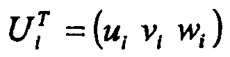
- Using the notation
- βi = dip angle (positive or negative)
- αi = azimuth for the dip angle direction
- The covariance matrix for a position is expressed as:

- For a multiple position vector this gives

- If Ui is a linear function of Xi like the orthogonal transformation:

then
- For a multiple point vector:

where
- The method is based on connecting the different systems through common points identified in both systems. The equations demonstrate the method for combining two models/systems denoted Wand G.
- We now introduce the following co-ordinate vectors concerning the common points:
- XW1 - Common points in system/model W
- XG1 - Common points in system/model G
- XL - Relative positions from sensor in W to recognised geological marker in G, i.e. result from a logging tool which senses remote geological markers, resistivity, acoustic reflectors, etc.
- The above vectors have the same dimension. An ideal match between the positions in the two systems gives:

- This equation also expresses the main constraint which ties the two systems together. When geological markers are observed directly, e.g. in a well, XL=0.
- Additionally we introduce:
- XW2 - Other points of interest in system/model W
- XG2 - Other points of interest in system/model G
- All the co-ordinate vectors are arranged like this:

with the corresponding covariance matrix, which is logically devided into sub-matrices, like this:
- The 0 matrices are considered to be unquestionable. Some of the other non-symmetric matrices may also be 0; however they are kept non-zero to allow generality.
- By using a generalized least squares methodology, the new vector and covariance matrices are calculated like this:


- The least squares solution results in an optimised tie between the two systems and points outside the common points are moved correctly according to their correlation to the tie-in points.
- The C1 and C0 matrices are dependent on which properties are to be achieved. The following solutions A and B are examples of realizations of two evident wanted properties. However, the way the models are constructed and the way data are organized make it possible to introduce any other wanted behaviour.
- The computer work can be reduced drastically by deriving optimised algorithms:
- using simplified algorithms for multiplication with unity matrices;
- omitting multiplications with zero matrices;
- reducing the dimension of the matrix to be inverted;
- utilizing quadratic forms of the expression.
- This solution gives the average position for the common points in the two systems. The other points, in both systems, will receive coordinate changes through the correlation.
- The C1 and the C0 matrices are identical:

D has a form and dimension dependent on the tie-in properties. - The 3D tie- in represents the situation where points can be identified and recognised in all directions (x, y, z). The matrix D becomes the unit matrix.


where - I
- - unit matrix (quadratic)
- 0
- - zero matrix
- n
- - number of common points, i.e. number of points in the vectors XW1 XG1 and XL
- k
- - number of points in XW2
- l
- - number of points in XG2
- This case occures where surfaces are identified. The tie is in force for the w direction only (perpendicular to the surface), and the D matrix comprises coefficients from the transformation from the X co-ordinate system to the U co-ordinate system.

- All submatrices in D have dimensions in the ratio 1:3. Then:

- In some situations, it may be desirable to keep one of the systems untouched. This means that the other system is transformed into the first system through the common points. Presupporting the W system to be held fixed, the C matrices are:

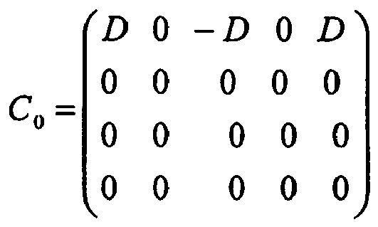
- The dimensions are still determined by the number of points in the different co-ordinate vectors:

where
and
- The dimensions in C0 are analogous to those in C1.
- The relative uncertainty between any pair of points in the X vector are determined by the general formula:

where B has the form:
- The unit matrices are placed logically in the right place according to the points of interest.
- This is a subject which is normally solved by solution B. The geological (G) model is transformed into the positions of the wellbore (W).
- The geological model is geometrically made up by a number of planes (geological boundaries). Each boundary is represented by one point in the plane and the dip angle and the azimuth in dip direction. When we recognize a geological marker (boundary) in the wellbore, we have only the information that we are in the boundary plane; not where. This means, mathematically, that we have a 1D tie-in, rather than a 3D tie-in.
-
Figure 5 illustrates a case where a well is being drilled to hit atarget 20 at ageological marker 21. However, thewellbore 22 will cross ageological marker 23 before thetarget 20 is reached. This gives the opportunity to have control of the positions in the geological model versus the positions in the wellbore before the critical phase (hitting the target) starts. Furthermore, the deviations of positions at themarker 23 in the two systems are utilised to enhance the positions and their accuracies in the geological model. - The following numerical example is simplified to deal with East and Vertical co-ordinates only. Furthermore, the L vector and its effect are removed in this calculation example.
- The geological marker 23 (dip angle = -3.0degree) is reached at a wellbore position that is 20m and 60m off the corresponding co-ordinates in the geological model.
- The collocation leads to the
geological markers target 20 at the geological marker 21 (and the associated wellbore co-ordinates) should therefore be changed to be identical to new co-ordinates forgeological marker 21. (It should be noted that the co-ordinates themselves do not become identical for the wellbore and geological models at thegeological marker 23. However, the geological marker surface goes through the actual wellbore position.) - The colloction further implies that the standard deviations for the relative position between geology and wellbore decreases from 106.65m to 106.11m in the East direction and decreases from 53.45m to 6.29m in the Vertical direction. The major enhancement in the Vertical direction is caused by the tie direction which is close to vertical (3 degree deflection).
Co-ordinates Standard deviations Before Collocation After Collocation Difference Before Collocation After Collocation Difference Wellbore E_1 1000.00 1000.00 0.00 11.00 11.00 0.00 V_1 2410.41 2410.41 0.00 4.92 4.92 0.00 E_2 1453.15 1453.15 0.00 11.52 11.52 0.00 V_2 2621.72 2621.72 0.00 5.66 5.66 0.00 Geology E_1 1020.00 1007.15 12.85 98.63 98.09 0.54 V_1 2470.41 2410.03 60.37 48.94 7.03 41.90 E_2 1453.15 1439.61 13.55 106.03 105.47 0.56 V_2 2621.72 2556.22 65.50 53.15 8.03 45.11 Difference Geology - wellbore E_1 20.00 7.15 12.85 V_1 60.00 -0.37 60.37 E_2 0.00 -13.55 13.55 106.65 106.11 0.54 V_2 0.00 -65.50 65.50 53.45 6.29 47.16 -
Figure 6 illustrates the originally plannedborehole 22 and the new borehole 22' after revising the position data following the intersection with themarker 23. The revised positions of the first and second markers are shown at 23' and 21' and the revised position of the target at 20'. - The matrix C1 is:
0.05 1.00 0.00 0.00 -0.05 -1.00 0.00 0.00 1.00 0.00 0.00 0.00 0.00 0.00 0.00 0.00 0.00 1.00 0.00 0.00 0.00 0.00 0.00 0.00 0.00 0.00 1.00 0.00 0.00 0.00 0.00 0.00 0.00 0.00 0.00 1.00 0.00 0.00 0.00 0.00 - The covariance matrix before collocation is:
W_E_1 W_V_1 W_E_2 W_V_2 G_E_1 G_V_1 G_E_2 G_V_2 W_E_1 120.90 -9.63 123.60 -12.17 0.00 0.00 0.00 0.00 W_V_1 -9.63 24.21 -11.99 27.21 0.00 0.00 0.00 0.00 W_E_2 123.60 -11.99 132.74 -15.22 0.00 0.00 0.00 0.00 W_V_2 -12.17 27.21 -15.22 32.08 0.00 0.00 0.00 0.00 G_E_1 0.00 0.00 0.00 0.00 9727.74 0.00 10251.68 0.00 G_V_1 0.00 0.00 0.00 0.00 0.00 2394.76 0.00 2598.00 G_E_2 0.00 0.00 0.00 0.00 10251.68 0.00 11241.63 0.00 G_V_2 0.00 0.00 0.00 0.00 0.00 2598.00 0.00 2824.85 - The covariance matrix after collocation is:
W_E_1 W_V_1 W_E_2 W_V_2 G_E_1 G_V_1 G_E_2 G_V_2 W_E_1 120.90 -9.63 123.60 -12.17 -0.69 -3.26 -0.73 -3.54 W_V_1 -9.63 24.21 -11.99 27.21 4.99 23.44 5.26 25.43 W_E_2 123.60 -11.99 132.74 -15.22 -1.16 -5.45 -1.22 -5.91 W_V_2 -12.17 27.21 -15.22 32.08 5.59 26.28 5.90 28.51 G_E_1 -0.69 4.99 -1.16 5.59 9621.45 -499.28 10139.67 -541.66 G_V_1 -3.26 23.44 -5.45 26.28 -499.28 49.44 -526.18 53.64 G_E_2 -0.73 5.26 -1.22 5.90 10139.67 -526.18 11123.59 -570.83 G_V_2 -3.54 25.43 -5.91 28.51 -541.66 53.64 -570.83 64.55 - Such a method may be characterised by:
- The core method is point-based (3 D), i.e. cells in a gridded geological model.
- Least squares estimation which supports both un-correlated and correlated observations with different weights.
- Flexible with respect to tie-on mechanisms by using appropriate constraints.
- Geological models described by zones between geological boundaries (geological markers) are reformulated into the point-based scheme before applying the general methodology.
- Correlation properties are represented by covariances rather than separate parameters.
- Typical applications include:
- Combination of any geological and/or petrophysical models into one common and unified model.
- Updating geological models with log information (detection of markers) which are measured in a wellbore.
- Calculation of relative positions and uncertainties for the purpose of targeting oil/gas reservoir zones.
- The achievements of using the method can be described by:
- Collocating all geological/petrophysical information into one unified model in the most optimal way. The result is a model with the overall lowest position uncertainties
- Optimising drilling program and targeting of oil/gas reservoirs, i.e. increasing hitting probabilities.


where

and ΔUi is the position of the X system origin in the U system and ΔXi is the position of the U system origin in the X system. Thus:

Claims (24)
- A method of combining at least two physical models based on measurements of a common region of the earth to form a resultant model, in which the positions and the positional uncertainties of at least one common point (CP1a - CP4a, CP1b - CP4b)in the at least two models are known, comprising deriving a position and a positional uncertainty in the resultant model of the at least one common point (CP1a - CP4a, CP1b - CP4b) from the positions and the positional uncertainties of the at least one common point (CP1a - CP4a, CP1b - CP4b) in the at least two models.
- A method as claimed in claim 1, characterised in that the positional uncertainties are represented as variances and covariances.
- A method as claimed in claim 1 or 2, characterised in that a first of the at least two models is a geological model.
- A method as claimed in claim 3, characterised in that the geological model is based on at least one of seismic, magnetometer and gravity measurements.
- A method as claimed in claim 3 or 4, characterised in that a second of the at least two models is based on wellbore log information.
- A method as claimed in any one of the preceding claims, characterised in that the at least one common point comprises a plurality of common points (CP1a - CP4a, CP1b - CP4b).
- A method as claimed in any one of the preceding claims, characterised in that a predetermined positional relationship exists between the position of at least one point of interest (PI1a - PI3a) in a or the first of the at least two models and the position of the at least one common point (CP1a - CP4a, CP1b - CP4b) in the first model and the position (PI1c - PI3c) of the at least one point of interest in the resultant model is derived from the position of the at least one common point (CP1c - CP4c) in the resultant model and from the predetermined positional relationship.
- A method as claimed in claim 7, characterised in that the at least one point of interest comprises a plurality of points of interest (PI1a - PI3a).
- A method as claimed in claim 7 or 8, characterised in that the predetermined positional relationship is represented as a correlation.
- A method as claimed in claim 7 or 8, characterised in that the predetermined positional relationship is represented as covariances.
- A method as claimed in any one of claims 7 to 10, characterised in that the predetermined positional relationship is a function of position.
- A method as claimed in claim 11, characterised in that the predetermined positional relationship is a decreasing function of distance between the at least one common point (CP1a - CP4a) and the at least one point of interest (PI1a - PI3a).
- A method as claimed in claim 11 or 12, characterised in that the predetermined positional relationship is a decreasing function of measurement noise between the at least one common point (CP1a - CP4a) and the at least one point of interest (PI1a - PI3a).
- A method as claimed in any one of claims 7 to 13, characterised in that a further predetermined positional relationship exists between the position of the at least one common point (CP1b - CP4b) in a or the second of the at least two models and the position of at least one further point of interest in the second model, the method comprising deriving a position in the third model of the at least one further point of interest from the position of the at least one common point (CP1c - CP4c) in the third model and from the further predetermined positional relationship.
- A method as claimed in any one of claims 7 to 14, characterised in that the position of the at least one common point (CP1c - CP4c) in the resultant model is the same as the position of the at least one common point in a or the second of the at least two models.
- A method as claimed in any one of the preceding claims, characterised by generating a or the second of the at least two models progessively and forming the resultant model upon the appearance in the second model of a first of the common points.
- A method as claimed in claim 16, characterised by replacing a or the first of the at least two models with the previously formed resultant model and forming a new resultant model each time a further one of the common points appears in the second model.
- A method as claimed in claim 17, characterised in that at least one portion of the new resultant model containing at least one common point which has previously appeared is unchanged when the new resultant model is formed.
- A method as claimed in claim 18, characterised in that the further one of the common points is in a surface and the at least one unchanged portion is a volume bounded by the surface.
- A method as claimed in any one of claims 16 to 19, characterised in that the first model is a geological model and the second model is generated during drilling of a wellbore.
- A method as claimed in claim 20 when dependent on claim 19, characterised in that the surface is a boundary between different layers and the appearance of the further one of the common points is indicated when the borehole penetrates the boundary.
- A computer program comprising computer readable code which, when run on a computer device, causes the computer device to perform a method as claimed in any one of the preceding claims.
- A medium containing a computer program as claimed in claim 22.
- A computer device programmed by a computer program as claimed in claim 22.
Applications Claiming Priority (2)
| Application Number | Priority Date | Filing Date | Title |
|---|---|---|---|
| GBGB0125713.8A GB0125713D0 (en) | 2001-10-26 | 2001-10-26 | Method of combining spatial models |
| GB0125713 | 2001-10-26 |
Publications (3)
| Publication Number | Publication Date |
|---|---|
| EP1306694A2 EP1306694A2 (en) | 2003-05-02 |
| EP1306694A3 EP1306694A3 (en) | 2004-07-21 |
| EP1306694B1 true EP1306694B1 (en) | 2014-03-19 |
Family
ID=9924571
Family Applications (1)
| Application Number | Title | Priority Date | Filing Date |
|---|---|---|---|
| EP02102465.8A Expired - Lifetime EP1306694B1 (en) | 2001-10-26 | 2002-10-18 | Method of combining spatial models |
Country Status (5)
| Country | Link |
|---|---|
| US (1) | US7149672B2 (en) |
| EP (1) | EP1306694B1 (en) |
| DK (1) | DK1306694T3 (en) |
| GB (1) | GB0125713D0 (en) |
| NO (1) | NO333785B1 (en) |
Families Citing this family (18)
| Publication number | Priority date | Publication date | Assignee | Title |
|---|---|---|---|---|
| GB2409900B (en) | 2004-01-09 | 2006-05-24 | Statoil Asa | Processing seismic data representing a physical system |
| GB2420855B (en) | 2004-12-02 | 2009-08-26 | Electromagnetic Geoservices As | Source for electromagnetic surveying |
| GB2435693A (en) | 2006-02-09 | 2007-09-05 | Electromagnetic Geoservices As | Seabed electromagnetic surveying |
| GB2439378B (en) | 2006-06-09 | 2011-03-16 | Electromagnetic Geoservices As | Instrument for measuring electromagnetic signals |
| GB2442749B (en) | 2006-10-12 | 2010-05-19 | Electromagnetic Geoservices As | Positioning system |
| GB2445582A (en) | 2007-01-09 | 2008-07-16 | Statoil Asa | Method for analysing data from an electromagnetic survey |
| WO2012086824A1 (en) * | 2010-12-20 | 2012-06-28 | 日本電気株式会社 | Operation management device, operation management method, and program |
| GB2486877B (en) * | 2010-12-21 | 2018-02-07 | Statoil Petroleum As | Quality control of sub-surface and wellbore position data |
| CA2826854C (en) * | 2011-02-08 | 2016-02-02 | Schlumberger Canada Limited | Three-dimensional modeling of parameters for oilfield drilling |
| RU2600493C2 (en) | 2011-09-07 | 2016-10-20 | Бейкер Хьюз Инкорпорейтед | Device and method for determination of geological boundaries |
| US20140155084A1 (en) * | 2012-12-03 | 2014-06-05 | Qualcomm Incorporated | Multi-mode wireless position association |
| US10228987B2 (en) * | 2013-02-28 | 2019-03-12 | Baker Hughes, A Ge Company, Llc | Method to assess uncertainties and correlations resulting from multi-station analysis of survey data |
| US10400590B1 (en) * | 2015-10-16 | 2019-09-03 | Emerson Paradigm Holding Llc | Method and system for determining a distribution of rock types in geological cells around a wellbore |
| GB2556621B (en) * | 2016-09-30 | 2020-03-25 | Equinor Energy As | Improved structural modelling |
| US10520644B1 (en) | 2019-01-10 | 2019-12-31 | Emerson Paradigm Holding Llc | Imaging a subsurface geological model at a past intermediate restoration time |
| US11156744B2 (en) | 2019-01-10 | 2021-10-26 | Emerson Paradigm Holding Llc | Imaging a subsurface geological model at a past intermediate restoration time |
| US11572785B2 (en) | 2021-01-26 | 2023-02-07 | Saudi Arabian Oil Company | Drilling uncertainty real time updates for accurate well placement |
| US12509981B2 (en) | 2022-09-09 | 2025-12-30 | Saudi Arabian Oil Company | Parametric attribute of pore volume of subsurface structure from structural depth map |
Family Cites Families (14)
| Publication number | Priority date | Publication date | Assignee | Title |
|---|---|---|---|---|
| US4926394A (en) * | 1989-10-27 | 1990-05-15 | Western Atlas International, Inc. | Monte Carlo method for estimating lithology from seismic data |
| US5170440A (en) * | 1991-01-30 | 1992-12-08 | Nec Research Institute, Inc. | Perceptual grouping by multiple hypothesis probabilistic data association |
| US5581024A (en) * | 1994-10-20 | 1996-12-03 | Baker Hughes Incorporated | Downhole depth correlation and computation apparatus and methods for combining multiple borehole measurements |
| US6061412A (en) * | 1995-10-05 | 2000-05-09 | Westinghouse Electric Company Llc | Nuclear reaction protection system |
| US5838634A (en) | 1996-04-04 | 1998-11-17 | Exxon Production Research Company | Method of generating 3-D geologic models incorporating geologic and geophysical constraints |
| US5905657A (en) | 1996-12-19 | 1999-05-18 | Schlumberger Technology Corporation | Performing geoscience interpretation with simulated data |
| US6549854B1 (en) * | 1999-02-12 | 2003-04-15 | Schlumberger Technology Corporation | Uncertainty constrained subsurface modeling |
| FR2792419B1 (en) * | 1999-04-16 | 2001-09-07 | Inst Francais Du Petrole | METHOD FOR OBTAINING AN OPTIMAL MODEL OF A PHYSICAL CHARACTERISTICS IN A HETEROGENEOUS ENVIRONMENT, SUCH AS THE BASEMENT |
| US6826483B1 (en) * | 1999-10-13 | 2004-11-30 | The Trustees Of Columbia University In The City Of New York | Petroleum reservoir simulation and characterization system and method |
| FR2800473B1 (en) * | 1999-10-29 | 2001-11-30 | Inst Francais Du Petrole | METHOD FOR 2D OR 3D MODELING A HETEROGENEOUS MEDIUM SUCH AS THE BASEMENT DESCRIBED BY SEVERAL PHYSICAL PARAMETERS |
| US6480790B1 (en) | 1999-10-29 | 2002-11-12 | Exxonmobil Upstream Research Company | Process for constructing three-dimensional geologic models having adjustable geologic interfaces |
| GB0018480D0 (en) * | 2000-07-27 | 2000-09-13 | Geco Prakla Uk Ltd | A method of processing surface seismic data |
| US6950786B1 (en) * | 2000-10-10 | 2005-09-27 | Schlumberger Technology Corporation | Method and apparatus for generating a cross plot in attribute space from a plurality of attribute data sets and generating a class data set from the cross plot |
| US20020120429A1 (en) * | 2000-12-08 | 2002-08-29 | Peter Ortoleva | Methods for modeling multi-dimensional domains using information theory to resolve gaps in data and in theories |
-
2001
- 2001-10-26 GB GBGB0125713.8A patent/GB0125713D0/en not_active Ceased
-
2002
- 2002-10-18 EP EP02102465.8A patent/EP1306694B1/en not_active Expired - Lifetime
- 2002-10-18 DK DK02102465.8T patent/DK1306694T3/en active
- 2002-10-22 US US10/277,616 patent/US7149672B2/en not_active Expired - Lifetime
- 2002-10-24 NO NO20025100A patent/NO333785B1/en not_active IP Right Cessation
Also Published As
| Publication number | Publication date |
|---|---|
| NO333785B1 (en) | 2013-09-16 |
| EP1306694A3 (en) | 2004-07-21 |
| US7149672B2 (en) | 2006-12-12 |
| US20030101033A1 (en) | 2003-05-29 |
| NO20025100L (en) | 2003-04-28 |
| DK1306694T3 (en) | 2014-06-16 |
| GB0125713D0 (en) | 2001-12-19 |
| EP1306694A2 (en) | 2003-05-02 |
| NO20025100D0 (en) | 2002-10-24 |
Similar Documents
| Publication | Publication Date | Title |
|---|---|---|
| US9164188B2 (en) | Forming a geological model | |
| US7149672B2 (en) | Method of combining spatial models | |
| RU2652172C2 (en) | Stratigraphic and structural interpretation of deviated and horizontal wellbores | |
| AU2017200089B2 (en) | System, method and computer program product for a rug plot for geosteering applications | |
| CN110073246B (en) | Improved method relating to quality control | |
| CN103370638A (en) | Quality control of sub-surface and wellbore position data | |
| Lesso Jr et al. | The principles and procedures of geosteering | |
| NO20190515A1 (en) | Improved structural modelling | |
| WO2022066289A1 (en) | Borehole localization relative to objects and subterranean formations | |
| WO1996035859A1 (en) | A process for directional drilling | |
| Shao et al. | Study of real-time LWD data visual interpretation and geo-steering technology | |
| US12497886B2 (en) | Three-dimensional reservoir mapping for drilling hydrocarbon wells | |
| US12436310B2 (en) | Reservoir properties derived using ultra-deep resistivity inversion data | |
| US20240004101A1 (en) | Analyzing borehole paths using stratigraphic turning points | |
| WO2006106337A1 (en) | Seismic data positioning | |
| Gangemi et al. | Integration of directional survey uncertainty in structural modelling: from geo-steering activities to geological interpretation | |
| Antonov et al. | Maximizing Net Pay in Penta-Lateral Well With Advanced Proactive Geosteering and 2D Structural Analysis Using Azimuthal Resistivity Measurements | |
| Pesenti et al. | Geological modelling workflow to support well placement: a case study from Barents Sea | |
| Fernandes et al. | 3D probabilistic well-log analysis with uncertain location data | |
| Jackson et al. | Field implementation of geological steering techniques optimizes drilling in highly-deviated and horizontal wells | |
| CN121365493A (en) | Geological modeling method and device, electronic equipment and readable storage medium | |
| McInerney et al. | Using airborne gravity data to better define the 3D limestone distribution at the Bwata Gas Field, Papua New Guinea | |
| Bybee | Updating a real-time 3D Earth model while drilling a horizontal well |
Legal Events
| Date | Code | Title | Description |
|---|---|---|---|
| PUAI | Public reference made under article 153(3) epc to a published international application that has entered the european phase |
Free format text: ORIGINAL CODE: 0009012 |
|
| AK | Designated contracting states |
Designated state(s): AT BE BG CH CY CZ DE DK EE ES FI FR GB GR IE IT LI LU MC NL PT SE SK TR |
|
| AX | Request for extension of the european patent |
Extension state: AL LT LV MK RO SI |
|
| PUAL | Search report despatched |
Free format text: ORIGINAL CODE: 0009013 |
|
| AK | Designated contracting states |
Kind code of ref document: A3 Designated state(s): AT BE BG CH CY CZ DE DK EE ES FI FR GB GR IE IT LI LU MC NL PT SE SK TR |
|
| AX | Request for extension of the european patent |
Extension state: AL LT LV MK RO SI |
|
| 17P | Request for examination filed |
Effective date: 20041213 |
|
| AKX | Designation fees paid |
Designated state(s): AT BE BG CH CY CZ DE DK EE ES FI FR GB GR IE IT LI LU MC NL PT SE SK TR |
|
| 17Q | First examination report despatched |
Effective date: 20090615 |
|
| RAP1 | Party data changed (applicant data changed or rights of an application transferred) |
Owner name: STATOIL PETROLEUM AS |
|
| GRAP | Despatch of communication of intention to grant a patent |
Free format text: ORIGINAL CODE: EPIDOSNIGR1 |
|
| INTG | Intention to grant announced |
Effective date: 20131009 |
|
| GRAS | Grant fee paid |
Free format text: ORIGINAL CODE: EPIDOSNIGR3 |
|
| GRAA | (expected) grant |
Free format text: ORIGINAL CODE: 0009210 |
|
| AK | Designated contracting states |
Kind code of ref document: B1 Designated state(s): AT BE BG CH CY CZ DE DK EE ES FI FR GB GR IE IT LI LU MC NL PT SE SK TR |
|
| REG | Reference to a national code |
Ref country code: GB Ref legal event code: FG4D |
|
| REG | Reference to a national code |
Ref country code: CH Ref legal event code: EP |
|
| REG | Reference to a national code |
Ref country code: IE Ref legal event code: FG4D |
|
| REG | Reference to a national code |
Ref country code: AT Ref legal event code: REF Ref document number: 658024 Country of ref document: AT Kind code of ref document: T Effective date: 20140415 |
|
| REG | Reference to a national code |
Ref country code: DE Ref legal event code: R096 Ref document number: 60246091 Country of ref document: DE Effective date: 20140430 |
|
| REG | Reference to a national code |
Ref country code: DK Ref legal event code: T3 Effective date: 20140610 |
|
| REG | Reference to a national code |
Ref country code: NL Ref legal event code: VDEP Effective date: 20140319 |
|
| REG | Reference to a national code |
Ref country code: AT Ref legal event code: MK05 Ref document number: 658024 Country of ref document: AT Kind code of ref document: T Effective date: 20140319 |
|
| PG25 | Lapsed in a contracting state [announced via postgrant information from national office to epo] |
Ref country code: FI Free format text: LAPSE BECAUSE OF FAILURE TO SUBMIT A TRANSLATION OF THE DESCRIPTION OR TO PAY THE FEE WITHIN THE PRESCRIBED TIME-LIMIT Effective date: 20140319 Ref country code: SE Free format text: LAPSE BECAUSE OF FAILURE TO SUBMIT A TRANSLATION OF THE DESCRIPTION OR TO PAY THE FEE WITHIN THE PRESCRIBED TIME-LIMIT Effective date: 20140319 Ref country code: CY Free format text: LAPSE BECAUSE OF FAILURE TO SUBMIT A TRANSLATION OF THE DESCRIPTION OR TO PAY THE FEE WITHIN THE PRESCRIBED TIME-LIMIT Effective date: 20140319 |
|
| PG25 | Lapsed in a contracting state [announced via postgrant information from national office to epo] |
Ref country code: BE Free format text: LAPSE BECAUSE OF FAILURE TO SUBMIT A TRANSLATION OF THE DESCRIPTION OR TO PAY THE FEE WITHIN THE PRESCRIBED TIME-LIMIT Effective date: 20140319 Ref country code: CZ Free format text: LAPSE BECAUSE OF FAILURE TO SUBMIT A TRANSLATION OF THE DESCRIPTION OR TO PAY THE FEE WITHIN THE PRESCRIBED TIME-LIMIT Effective date: 20140319 Ref country code: EE Free format text: LAPSE BECAUSE OF FAILURE TO SUBMIT A TRANSLATION OF THE DESCRIPTION OR TO PAY THE FEE WITHIN THE PRESCRIBED TIME-LIMIT Effective date: 20140319 Ref country code: NL Free format text: LAPSE BECAUSE OF FAILURE TO SUBMIT A TRANSLATION OF THE DESCRIPTION OR TO PAY THE FEE WITHIN THE PRESCRIBED TIME-LIMIT Effective date: 20140319 Ref country code: BG Free format text: LAPSE BECAUSE OF FAILURE TO SUBMIT A TRANSLATION OF THE DESCRIPTION OR TO PAY THE FEE WITHIN THE PRESCRIBED TIME-LIMIT Effective date: 20140619 |
|
| PG25 | Lapsed in a contracting state [announced via postgrant information from national office to epo] |
Ref country code: SK Free format text: LAPSE BECAUSE OF FAILURE TO SUBMIT A TRANSLATION OF THE DESCRIPTION OR TO PAY THE FEE WITHIN THE PRESCRIBED TIME-LIMIT Effective date: 20140319 Ref country code: ES Free format text: LAPSE BECAUSE OF FAILURE TO SUBMIT A TRANSLATION OF THE DESCRIPTION OR TO PAY THE FEE WITHIN THE PRESCRIBED TIME-LIMIT Effective date: 20140319 Ref country code: AT Free format text: LAPSE BECAUSE OF FAILURE TO SUBMIT A TRANSLATION OF THE DESCRIPTION OR TO PAY THE FEE WITHIN THE PRESCRIBED TIME-LIMIT Effective date: 20140319 |
|
| REG | Reference to a national code |
Ref country code: DE Ref legal event code: R097 Ref document number: 60246091 Country of ref document: DE |
|
| PG25 | Lapsed in a contracting state [announced via postgrant information from national office to epo] |
Ref country code: PT Free format text: LAPSE BECAUSE OF FAILURE TO SUBMIT A TRANSLATION OF THE DESCRIPTION OR TO PAY THE FEE WITHIN THE PRESCRIBED TIME-LIMIT Effective date: 20140721 |
|
| PLBE | No opposition filed within time limit |
Free format text: ORIGINAL CODE: 0009261 |
|
| STAA | Information on the status of an ep patent application or granted ep patent |
Free format text: STATUS: NO OPPOSITION FILED WITHIN TIME LIMIT |
|
| 26N | No opposition filed |
Effective date: 20141222 |
|
| PG25 | Lapsed in a contracting state [announced via postgrant information from national office to epo] |
Ref country code: IT Free format text: LAPSE BECAUSE OF FAILURE TO SUBMIT A TRANSLATION OF THE DESCRIPTION OR TO PAY THE FEE WITHIN THE PRESCRIBED TIME-LIMIT Effective date: 20140319 |
|
| REG | Reference to a national code |
Ref country code: DE Ref legal event code: R097 Ref document number: 60246091 Country of ref document: DE Effective date: 20141222 |
|
| REG | Reference to a national code |
Ref country code: DE Ref legal event code: R119 Ref document number: 60246091 Country of ref document: DE |
|
| PG25 | Lapsed in a contracting state [announced via postgrant information from national office to epo] |
Ref country code: MC Free format text: LAPSE BECAUSE OF FAILURE TO SUBMIT A TRANSLATION OF THE DESCRIPTION OR TO PAY THE FEE WITHIN THE PRESCRIBED TIME-LIMIT Effective date: 20140319 Ref country code: LU Free format text: LAPSE BECAUSE OF FAILURE TO SUBMIT A TRANSLATION OF THE DESCRIPTION OR TO PAY THE FEE WITHIN THE PRESCRIBED TIME-LIMIT Effective date: 20141018 |
|
| REG | Reference to a national code |
Ref country code: CH Ref legal event code: PL |
|
| REG | Reference to a national code |
Ref country code: IE Ref legal event code: MM4A |
|
| PG25 | Lapsed in a contracting state [announced via postgrant information from national office to epo] |
Ref country code: LI Free format text: LAPSE BECAUSE OF NON-PAYMENT OF DUE FEES Effective date: 20141031 Ref country code: CH Free format text: LAPSE BECAUSE OF NON-PAYMENT OF DUE FEES Effective date: 20141031 Ref country code: DE Free format text: LAPSE BECAUSE OF NON-PAYMENT OF DUE FEES Effective date: 20150501 |
|
| REG | Reference to a national code |
Ref country code: FR Ref legal event code: ST Effective date: 20150630 |
|
| PG25 | Lapsed in a contracting state [announced via postgrant information from national office to epo] |
Ref country code: FR Free format text: LAPSE BECAUSE OF NON-PAYMENT OF DUE FEES Effective date: 20141031 |
|
| PG25 | Lapsed in a contracting state [announced via postgrant information from national office to epo] |
Ref country code: IE Free format text: LAPSE BECAUSE OF NON-PAYMENT OF DUE FEES Effective date: 20141018 |
|
| PG25 | Lapsed in a contracting state [announced via postgrant information from national office to epo] |
Ref country code: GR Free format text: LAPSE BECAUSE OF FAILURE TO SUBMIT A TRANSLATION OF THE DESCRIPTION OR TO PAY THE FEE WITHIN THE PRESCRIBED TIME-LIMIT Effective date: 20140620 |
|
| PG25 | Lapsed in a contracting state [announced via postgrant information from national office to epo] |
Ref country code: TR Free format text: LAPSE BECAUSE OF FAILURE TO SUBMIT A TRANSLATION OF THE DESCRIPTION OR TO PAY THE FEE WITHIN THE PRESCRIBED TIME-LIMIT Effective date: 20140319 |
|
| PGFP | Annual fee paid to national office [announced via postgrant information from national office to epo] |
Ref country code: DK Payment date: 20191024 Year of fee payment: 18 |
|
| REG | Reference to a national code |
Ref country code: DK Ref legal event code: EBP Effective date: 20201031 |
|
| PG25 | Lapsed in a contracting state [announced via postgrant information from national office to epo] |
Ref country code: DK Free format text: LAPSE BECAUSE OF NON-PAYMENT OF DUE FEES Effective date: 20201031 |
|
| PGFP | Annual fee paid to national office [announced via postgrant information from national office to epo] |
Ref country code: GB Payment date: 20211026 Year of fee payment: 20 |
|
| REG | Reference to a national code |
Ref country code: GB Ref legal event code: PE20 Expiry date: 20221017 |
|
| PG25 | Lapsed in a contracting state [announced via postgrant information from national office to epo] |
Ref country code: GB Free format text: LAPSE BECAUSE OF EXPIRATION OF PROTECTION Effective date: 20221017 |