Technical Field
-
This invention relates a fractal structure
and its forming method, especially based on a novel
principle.
Background Art
-
For application of a solid material to
electronic or optical devices, physical properties of
the material may restrict its applications. For
example, in case of using a semiconductor material in a
light emitting device, it will be usable in a device of
an emission wavelength corresponding to the band gap of
the material, but some consideration will be necessary
for changing the emission wavelength. Regarding
physical properties related to semiconductor bands,
controls by superlattices have been realized. More
specifically, by changing the period of a superlattice,
the bandwidth of its subband can be controlled to
design an emission wavelength.
-
Targeting on controlling many-electron-state
structures by material designs, the Inventor proposed
many-body effect engineering by quantum dot-based
structures and has continued theoretical analyses ((1)
U.S. Patent 5,430,309; (2) U.S. Patent 5,663,571; (3)
U.S. Patent 5,719,407; (4) U.S. Patent 5,828,090; (5)
U.S. Patent 5,831,294; (6) U.S. Patent 6,020,605; (7)
J. Appl. Phys. 76, 2833(1994); (8) Phys. Rev. B51,
10714(1995); (9) Phys. Rev. B51, 11136(1995); (10) J.
Appl. Phys. 77, 5509(1995); (11) Phys. Rev. B53,
6963(1996); (12) Phys. Rev. B53, 10141(1996); (13)
Appl. Phys. Lett. 68, 2657(1996); (14) J. Appl. Phys.
80, 3893(1996); (15) J. Phys. Soc. Jpn. 65, 3952(1996);
(16) Jpn. J. Appl. Phys. 36, 638(1997); (17) J. Phys.
Soc. Jpn. 66, 425(1997); (18) J. Appl. Phys. 81, 2693
(1997); (19) Physica (Amsterdam) 229B, 146(1997); (20)
Physica (Amsterdam) 237A, 220(1997); (21) Surf. Sci.
375, 403(1997); (22) Physica (Amsterdam) 240B,
116(1997); (23) Physica (Amsterdam) 240B, 128(1997);
(24) Physica (Amsterdam) IE, 226(1997); (25) Phys. Rev.
Lett. 80, 572(1998); (26) Jpn. J. Appl. Phys. 37,
863(1998); (27) Physica (Amsterdam) 245B, 311(1998);
(28) Physica (Amsterdam) 235B, 96(1998); (29) Phys.
Rev. B59, 4952(1999); (30) Surf. Sci. 432, 1(1999);
(31) International Journal of Modern Physics B. Vol.
13, No. 21, 22, pp. 2689-2703, 1999). For example,
realization of various correlated electronic systems is
expected by adjusting a tunneling phenomenon between
quantum dots and interaction between electrons in
quantum dots. Let the tunneling transfer between
adjacent quantum dots be written as t. Then, if
quantum dots are aligned in form of a tetragonal
lattice, the bandwidth of one electron state is Teff=4t.
If quantum dots form a one-dimensional chain, the
bandwidth of one electron state is Teff=2t. In case of
a three-dimensional quantum dot array, Teff=6t. That
is, if D is the dimension of a quantum dot array, the
bandwidth of one electron state has been Teff=2Dt. Here
is made a review about half-filled (one electron per
each quantum dot) Mott transition (also-called Mott-Hubbard
transition or Mott metal-insulator transition).
Let the effective interaction of electrons within a
quantum dot be written as Ueff, then the Hubbard gap on
the part of the Mott insulator is substantially
described as Δ=Ueff-Teff, and the Mott transition can be
controlled by changing Ueff or t. As already proposed,
the Mott-Hubbard transition can be controlled by
adjusting Ueff or t, using a field effect, and it is
applicable to field effect devices (Literatures (5),
(6), (11) and (14) introduced above).
-
On the other hand, reviewing the equation of
Δ=Ueff-Teff=Ueff-2Dt, it will be possible to control
Mott-Hubbard transition by controlling the
dimensionality D of the system. For this purpose, the
Applicant already proposed a fractal-based structure
that can continuously change the dimensionality, and
have exhibited that Mott-Hubbard transition is
controllable by changing the fractal dimensions.
-
To enable designing of wider materials, it is
desired to modify and control the dimension of
materials by designing methods beyond the simple
fractal nature.
-
As physical systems in charge of information
processing, intrinsic non-linearity is indispensable.
As devices having been used for years, there are
electronic devices using materials exhibiting non-linear
responses to certain extents. For example, two-terminal
devices exhibiting differential negative
resistances are one example of devices that are non-linear
in current-voltage characteristics. Of course,
MOS-FET, which is a three-terminal device, supports the
modern technologies. By coupling these electronic
devices having non-linear properties with a linear
electronic circuit and constructing an information
processing device having a non-linear property, any
desired calculation can be executed.
-
However, difficulties by high integration
have become issues with such electronic circuits.
Generation of heat is one of the problems, for example.
The heat generation caused by intrinsic electric
resistance is mandatory for producing non-linearity of
an electronic device, and indispensable and essential
for executing information processing.
-
To avoid this difficulty, trials have been
made to decrease the number of devices by enhancing
non-linearity of component devices. Progress of this
scheme necessarily results in the need for component
devices having non-linearity as strong as chaotic.
When a chaotic classical system is quantized, what
characterizes the behaviors of the quantum system is
quantum chaos.
-
On the other hand, as miniaturization of
component devices progresses, electrons confined in a
device result in behaving as quantum mechanical
particles. Therefore, from this point of view, hopes
are placed on components devices exhibiting quantum
chaos. The Applicant has continued to theoretically
demonstrate that, in a quantum system in a structure
having a fractal configuration, the quantum chaos can
be controlled by changing the fractal dimension
characterizing the system.
-
An object the invention intends to accomplish
is to provide a fractal structure and its forming
method capable of modulating and controlling the
dimensionality of a material by a design method beyond
the simple fractal nature.
-
Another object the invention intends to
accomplish is to provide a fractal structure and its
forming method capable of controlling phase transition
and chaos, in particular, quantum chaos, by a design
method beyond the simple fractal nature.
Disclosure of Invention
-
The Inventor found, through concentrated
researches toward solution of those issues, that a more
complex fractal structure having a portion
characterized by a plurality of fractal dimensions can
be formed by changing the growth conditions with time
during growth of the fractal structure. Especially in
the process of growing a random fractal, it has been
found that a fractal structure in form of nerve cells
can be formed by forming a region with a low fractal
dimension around a core with a high fractal dimension.
Then, it has been found that, in fractal structures of
this type, occurrence of phase transition, such as
magnetic phase transition, and chaos, such as quantum
chaos in an electron state, can be controlled. As a
result of later detailed analysis, it has been found
that there are fractal dimensions suitable for
controlling these phenomena.
-
The present invention has been made on the
basis of those researches by the Inventor.
-
That is, to overcome the above-indicated
problems, according to the first aspect of the
invention, there is provided a fractal structure
comprising a plurality of regions different in fractal
dimension characterizing the self-similarity.
-
In the first aspect of the invention, nature
of phase transition occurring in a fractal structure is
controlled by adjusting the ratios in volume of a
plurality of regions relative to the entire fractal
structure. Alternatively, correlation between
interactive electrons in an electron system is
controlled. Additionally, the magnetization curve of
ferromagnetic phase transition is controlled. Further,
nature of the chaos appearing in the fractal structure
is controlled, more specifically, the quantum chaos in
electrons states, for example, is controlled. Control
of the quantum chaos in electron states can be
controlled with a high controllability by using
introduction of a random magnetic field by addition of
a magnetic impurity in addition to adjustment of the
ratios in volume of a plurality of regions relative to
the entire fractal structure. Of course, control of
the quantum chaos in electron states is possible merely
by introducing a random magnetic field by addition of a
magnetic impurity without adjustment of the ratios in
volume of a plurality of regions relative to the entire
fractal structure. The ratios in volume of these
regions correspond to the ratios of numbers of atoms
forming these regions, and in embodiments of the
invention explained later, they correspond to the
ratios of durations of time for growth (step) required
for forming these regions.
-
In the first aspect of the invention, the
fractal structure typically includes a first region
forming the core having a first fractal dimension, and
one or more second regions surrounding the first region
and having a second fractal dimension that is lower
than the first fractal dimension. In the case where
the entirety of the first region and the second region
appears like a star, it is a stellar fractal structure.
In the fractal structure having these first and second
regions, from the viewpoint of ensuring sufficient
controllability of the nature of phase transition or
correlation between interactive electrons in an
electron system, that is, from the viewpoint of forming
a satisfactory junction between a Mott insulator and a
metal by satisfactorily controlling the magnetization
curve of ferromagnetic phase transition, quantum chaos,
and so on, or by satisfactorily forming Df1 and the
second fractal dimension Df2 are determined to be
preferably Df1>2.7 and Df2<2.3, typically 2.7<Df1≦3
and 1≦Df2<2.3, and more preferably 2.9≦Df1≦3 and 1≦
Df2<2.3. The upper limit value 3 of Df1 corresponds to
the dimension of a three-dimensional space whereas the
lower limit value 1 of Df2 is necessary for ensuring
connectivity in the structure.
-
According to the second aspect of the
invention, there is provided a method of forming a
fractal structure having a plurality of regions
different in fractal dimension characterizing the self-similarity,
comprising:
- growing a fractal structure from one or more
origins, and changing growth conditions with time in
the growth process thereof such that different fractal
dimensions are obtained.
-
-
In the second aspect of the invention, there
are used growth conditions ensuring the first fractal
dimension to be made from the growth start point of
time until a first point of time, and growth conditions
ensuring a second fractal dimension lower than-the
first fractal dimension to be made from the first point
of time to a second point of time. This results in
forming a fractal structure including a first region
having the first fractal dimension and a second region
surrounding the first region and having the second
fractal dimension lower than the first fractal
dimension. In an embodiment that will be explained
later in detail, growth conditions of the fractal
structure are represented by α of Equation (4). In
actual growth, however, if the fractal structure is
grown in the liquid phase, for example, natures of
solvents employed for the growth are one of the growth
conditions. That is, in this case, a plurality of
regions different in fractal dimension can be formed by
selecting appropriate solvents, respectively, in the
growth process.
-
Similarly to the first aspect of the
invention, in the fractal structure including the first
region and the second region, from the viewpoint of
ensuring sufficient controllability of the nature of
phase transition or correlation between interactive
electrons in an electron system, that is, from the
viewpoint of forming a satisfactory junction between a
Mott insulator and a metal by satisfactorily
controlling the magnetization curve of ferromagnetic
phase transition, quantum chaos, and so on, or by
satisfactorily forming Df1 and the second fractal
dimension Df2 are determined to be preferably Df1>2.7
and Df2<2.3, typically 2.7<Df1≦3 and 1≦Df2<2.3, and
more preferably 2.9≦Df1≦3 and 1≦Df2<2.3. The upper
limit value 3 of Df1 corresponds to the dimension of a
three-dimensional space whereas the lower limit value 1
of Df2 is necessary for ensuring connectivity in the
structure.
-
According to the invention having the above-summarized
configuration, a fractal structure, such as
a stellar fractal structure, including a plurality of
regions different in fractal dimension from each other
can be obtained by changing the growth condition of the
fractal structure with time. Then, in this fractal
structure, the nature of phase transition occurring in
the fractal structure can be controlled by adjusting
the ratios in volume of the plurality of regions
relative to the entire fractal structure. Optimization
of the fractal dimensions also improves the
controllability.
Brief Description of Drawings
-
- Fig. 1 is a schematic diagram that shows a
stellar fractal structure obtained by simulation
according to the first embodiment of the invention;
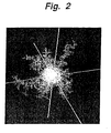
- Fig. 2 is a schematic diagram that shows a
stellar fractal structure obtained by simulation
according to the first embodiment of the invention;
- Fig. 3 is a schematic diagram for explaining
dimensions of a stellar fractal structure according to
the first embodiment;
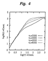
- Fig. 4 is a schematic diagram that shows log-log
plots of a distance r from the growth origin in the
stellar fractal structure according to the first
embodiment and the number of growth points N(r)
contained in a ball with the radius r;
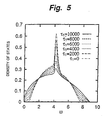
- Fig. 5 is a schematic diagram that shows a
relation between energy and density of states in the
stellar fractal structure according to the first
embodiment of the invention;
- Fig. 6 is a schematic diagram that shows a
relation between energy and density of states in the
stellar fractal structure according to the first
embodiment of the invention;
- Fig. 7 is a schematic diagram that shows a
relation between energy and density of states in the
stellar fractal structure according to the first
embodiment of the invention;
- Fig. 8 is a schematic diagram for explaining
spatial changes inside the stellar fractal structure
according to the first embodiment of the invention;
- Fig. 9 is a schematic diagram that shows log-log
plots of a distance r from the growth origin in a
stellar fractal structure according to the second
embodiment and the number of growth points N(r)
contained in a ball with the radius r;
- Fig. 10 is a schematic diagram that shows
log-log plots of a distance r from the growth origin in
a stellar fractal structure according to the second
embodiment and the number of growth points N(r)
contained in a ball with the radius r;
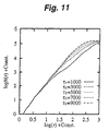
- Fig. 11 a schematic diagram that shows log-log
plots of a distance r from the growth origin in a
stellar fractal structure according to the second
embodiment and the number of growth points N(r)
contained in a ball with the radius r;
- Fig. 12 is a schematic diagram that shows
spontaneous magnetization in a fractal structure having
a single fractal dimension;
- Fig. 13 is a schematic diagram that shows
spontaneous magnetization in a stellar fractal
structure according to the second embodiment of the
invention;
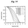
- Fig. 14 is a schematic diagram that shows
spontaneous magnetization in a stellar fractal
structure according to the second embodiment of the
invention;
- Fig. 15 is a schematic diagram that shows
spontaneous magnetization in a stellar fractal
structure according to the second embodiment of the
invention;
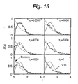
- Fig. 16 is a schematic diagram that shows
quantum level statistics in a stellar fractal structure
according to the third embodiment of the invention;
- Fig. 17 is a schematic diagram that shows
quantum level statistics in a stellar fractal structure
according to the third embodiment of the invention;
- Fig. 18 is a schematic diagram that shows
quantum level statistics in a stellar fractal structure
according to the third embodiment of the invention;
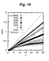
- Fig. 19 is a schematic diagram that shows
quantum level statistics in a stellar fractal structure
according to the third embodiment of the invention;
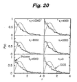
- Fig. 20 is a schematic diagram that shows
quantum level statistics in a stellar fractal structure
according to the third embodiment of the invention;
- Fig. 21 is a schematic diagram that shows
quantum level statistics in a stellar fractal structure
according to the third embodiment of the invention;
- Fig. 22 is a schematic diagram that shows
quantum level statistics in a stellar fractal structure
according to the fourth embodiment of the invention;
- Fig. 23 is a schematic diagram that shows
quantum level statistics in a stellar fractal structure
according to the fourth embodiment of the invention;
- Fig. 24 is a schematic diagram that shows
quantum level statistics in a stellar fractal structure
according to the fourth embodiment of the invention;
- Fig. 25 is a schematic diagram that shows
quantum level statistics in a stellar fractal structure
according to the fourth embodiment of the invention;
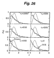
- Fig. 26 is a schematic diagram that shows
quantum level statistics in a stellar fractal structure
according to the fourth embodiment of the invention;
- Fig. 27 is a schematic diagram that shows
quantum level statistics in a stellar fractal structure
according to the fourth embodiment of the invention;
- Fig. 28 is a schematic diagram that shows a
relation between α and the fractal dimension Df in a
simplex fractal structure;
- Fig. 29 is a schematic diagram that shows
Ms(r) in a stellar fractal structure according to the
fifth embodiment of the invention;
- Fig. 30 is a schematic diagram that shows
Ms(r) in a stellar fractal structure according to the
fifth embodiment of the invention;
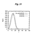
- Fig. 31 is a schematic diagram that shows
Ms(r) in a stellar fractal structure according to the
fifth embodiment of the invention;
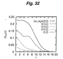
- Fig. 32 is a schematic diagram that shows
Dave(r) in a stellar fractal structure according to the
fifth embodiment of the invention;
- Fig. 33 is a schematic diagram that shows
Dave(r) in a stellar fractal structure according to the
fifth embodiment of the invention;
- Fig. 34 is a schematic diagram that shows
Dave(r) in a stellar fractal structure according to the
fifth embodiment of the invention;
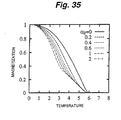
- Fig. 35 is a schematic diagram that shows
spontaneous magnetization in a stellar fractal
structure according to the sixth embodiment of the
invention;
- Fig. 36 is a schematic diagram that shows
spontaneous magnetization in a stellar fractal
structure according to the sixth embodiment of the
invention;
- Fig. 37 is a schematic diagram that shows
spontaneous magnetization in a stellar fractal
structure according to the sixth embodiment of the
invention;
- Fig. 38 is a schematic diagram that shows
spontaneous magnetization in a stellar fractal
structure according to the sixth embodiment of the
invention;
- Fig. 39 is a schematic diagram that shows
spontaneous magnetization in a stellar fractal
structure according to the sixth embodiment of the
invention;
- Fig. 40 is a schematic diagram that shows
spontaneous magnetization in a stellar fractal
structure according to the sixth embodiment of the
invention;
- Fig. 41 is a schematic diagram that shows
quantum level statistics in a stellar fractal structure
according to the seventh embodiment of the invention;
- Fig. 42 is a schematic diagram that shows
quantum level statistics in a stellar fractal structure
according to the seventh embodiment of the invention;
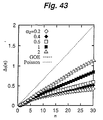
- Fig. 43 is a schematic diagram that shows
quantum level statistics in a stellar fractal structure
according to the seventh embodiment of the invention;
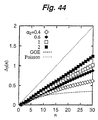
- Fig. 44 is a schematic diagram that shows
quantum level statistics in a stellar fractal structure
according to the seventh embodiment of the invention;
- Fig. 45 is a schematic diagram that shows
quantum level statistics in a stellar fractal structure
according to the seventh embodiment of the invention;
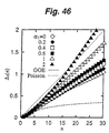
- Fig. 46 is a schematic diagram that shows
quantum level statistics in a stellar fractal structure
according to the seventh embodiment of the invention;
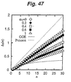
- Fig. 47 is a schematic diagram that shows
quantum level statistics in a stellar fractal structure
according to the seventh embodiment of the invention;
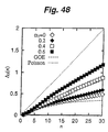
- Fig. 48 is a schematic diagram that shows
quantum level statistics in a stellar fractal structure
according to the seventh embodiment of the invention;
and
- Fig. 49 is a schematic diagram that shows the
Berry-Robnik parameter ρ in a star-shaped fractal
structure according to the seventh embodiment of the
invention.
-
Best Mode for Carrying Out the Invention
-
Some embodiments of the invention will now be
explained below. In the following embodiments, stellar
fractal structures are taken as one type of fractal
structures including a plurality of portions
characterized in a plurality of fractal dimensions.
These stellar fractal structures each have a form of a
nerve cell obtained by forming a region with a low
fractal dimension around a core with a high fractal
dimension in the process of growing random fractals.
First Embodiment
(1) Formation of a stellar fractal structure
-
A method of forming a stellar fractal
structure according to the first embodiment can be
obtained by developing Dielectric Breakdown Model ((32)
A. Erzan, L. Pietronero, A. Vespignani, Rev. Mod. Phys.
67, 545(1995); (33) L. Niemeyer, L. Pietronero, H.J.
Wiesmann, Phys. Rev. Lett. 52, 1033(1984)).
-
Here is defined a cubic lattice S in a three-dimensional
space, and a scalar potential field (i1,
i2, i3) is defined on its lattice site (i1, i2, i3)∈S
and called a potential. Let this potential obey the
Laplace's equation
Δ(i 1,i 2,i 3) = 0
A pattern Tn, which will be defined later, is a set of
lattice sites on the three-dimensional lattice. T0
contains (0, 0, 0) alone, and Tn+1 is created by
sequentially adding a single lattice site to Tn
according to the rule given below.
-
Let the potential of each site contained in
Tn be I and let the potential at infinity be 0. That
is,
(i 1,i 2,i 3)=0 when (i 1,i 2,i 3) → ∞
(i 1,i 2,i 3)=1 when (i 1,i 2,i 3)∈Tn
Under these boundary conditions, Equation (1) is solved
to determine the potential. The lattice site, which
will be added to Tn to construct Tn+1, is not contained
in Tn, and it is selected from the set of lattice
sites, i.e. Un, nearest to Tn. The number of lattice
sites contained in Un is denoted by Nn.
-
Intensity of the electric fields for lattice
sites (i
1,m, i
2,m, i
3,m) (where m=1, 2, ···, N
n) in U
n is
defined as
Em (α)= (i 1, m ,i 2, m ,i 3, m )-1 α
The probability that a certain site (i
1,m, i
2,m, i
3,m) in
U
n is selected is proportional to the electric field
E
m(α). That is, the probability is
-
By repeating these operations, construction
of T
n is progressed. An ideal fractal will be a set of
limits repeated infinitely as
When α=1, the foregoing and the result of generation
of the pattern by Diffusion limited aggregation are
consistent ((34) T.A. Witten, Jr. and L.M. Sander,
Phys. Rev. Lett. 47, 1400(1984); Phys. Rev. B 27,
5686(1983)).
-
The stellar fractal structure according to
the first embodiment is formed by changing the α
parameter in accordance with the step n of the above-mentioned
growth. That is, the above growth process is
progressed using α1 under 1≦n≦τ1, α2 under τ1+1≦n≦τ2,
and α3 under τ2+1≦n≦τ3. Simulation is performed below,
taking fractal structure having two different fractal
dimensions. Results of the simulation are shown in
Figs. 1, 2 and 3. In that simulation, τ2=10000, α1=0
and α2=2 are commonly used in all cases whereas τ1=3000
is used in Fig. 1, τ1=5000 is used in Fig. 2 and τ1=7000
is used in Fig. 3, respectively. It will be understood
from Figs. 1, 2 and 3 that the fractal structure
includes a ball-shaped region with a high fractal
dimension (somatic fractal) at the center (growth
origin) and a tree-like region with a low fractal
dimension (dendritic fractal) around it. Nerve cells
often exhibit this type of structure. That is, tree-like
projections extend from the soma of a cell and
perform their function.
-
For the purpose of understanding the
structure in greater detail, a calculation process of
fractal dimensions is used. Let r represent the
distance from the growth origin (0, 0, 0) and N(r)
represent the number of growth points contained in a
ball with the radius r. Then, using a as a factor of
proportionality, if N(r) can be expressed as
N(r)=arDf
then Df is called the fractal dimension. Therefore,
since logarithms of both sides are
logN(r) = loga + Df logr
if log-log plots ride on a straight line, the structure
can be regarded as a fractal, and its inclination is
the fractal dimension. In Fig. 4, log-log plotting was
made for various cases obtained by the above-mentioned
growth experiment. It is found from Fig. 4 that, under
a small log(r), plots ride on a straight line with a
large inclination, but they ride on a straight line
with a small inclination when log(r) exceeds a certain
critical point. This demonstrates that the structure
include two different fractal dimensions. More
specifically, in this example, the fractal dimension
before log(r) exceeds the critical point is
approximately 2.9, and excluding the case of τ1=8000,
the fractal dimension after log(r) exceeds the critical
point is approximately 2.1. Sites of the critical
point increase as τ1 increases, and this supports this
growth model and its interpretation.
(2) Correlative electron system in a stellar fractal
structure
-
An electron system is defined on the stellar
fractal structure defined in (1). A review is made
about the lattice point
rp = (i 1, pi 2, p ,i 3, p )∈Tn
that is the origin of T
n. In Equation (9), p=1, 2, ···,
n+1. An operator
C and † /
p,σ for generating an electron of a
spin σ is defined at the lattice point
rp ∈
Tn . Of
course, there is the anticommutative relation
Here is defined a single-band Hubbard Hamiltonian
H and of
the electron system as follows.
-
Assuming that electrons are movable only
among nearest-neighbor sites, the following is employed
as λ
p,q.
Additionally, the spin σ electron density operator of
the j-th site,
n andj ,σ =
c and ↑ /
j,σ
c andj ,σ, and their sum, n and
j = Σ
σ n andj ,σ,
are defined.
-
For the purpose of defining a temperature
Green's function, here is introduced a grand canonical
Hamiltonian
K and = H and - µN and where
N and = Σ
jn andj . In the half-filled
taken here, chemical potential is µ=U/2. The
half-filled grand canonical Hamiltonian can be
expressed as
Operators
t andj , i ,σ,
j andj , i ,σ,
ûi and
d andi ,σ are defined beforehand
as
t j,i,σ = c † j,σ c i,σ + c † i,σ c j,σ
j j,i,σ = c † j,σ c i,σ - c † i,σ c j,σ
û i = c † i,↑ c i,↑ c † i,↓ c i,↓ + c i,↑ c † i,↑ c i,↓ c † i,↓
d i,σ = c † i,σ c i,σ - c i,σ c † i,σ
If the temperature Green function is defined for
operators
 and
B and given, taking τ as imaginary time,
it is as follows.
The on-site Green function
G j,σ(iωn ) = 〈 c j,σ; c † j,σ〉
is especially important.
-
Imaginary time development of the system is
obtained by the Heisenberg equation
d dτ Â(τ) = [ K,Â]
As the equation of motion of the on-site Green
function,
is obtained. Then, the approximation shown below is
introduced, following Gros ((35) C. Gros, Phys. Rev.
B50, 7295(1994)). If the site p is the nearest-neighbor
site of the site j, the resolution
〈 c p,σ; c † j,σ〉 → t 〈 c p,σ; c † p,σ〉〈 c j,σ; c † j,σ〉
is introduced as the approximation. This is said to be
exact in case of infinite-dimensional Bethe lattices,
but in this case, it is only within approximation.
Under the approximation, the following equation is
obtained.
(iωn - t 2Γ j,σ )G j,σ = 1+ U 2 〈 d j,-σ c j,σ; c † j,σ〉
where
was introduced. To solve the equation, obtained,
〈
d andj ,-σ c andj ,σ;
c and † /
j,σ〉 has to be analyzed. In case of half-filled
models, this equation of motion is
Here again, with reference to the Gros theory,
approximation is introduced. It is the following
translation.
〈 j p,j,-σ c j,σ; c † j,σ〉 → -tGp,-σ 〈 d j,-σ c j,σ; c † j,σ〉
〈 d j,-σ c j,σ; c † j,σ〉 →tGp,σ 〈 d j,-σ c j,σ; c † j,σ〉
By executing this translation, the following closed
equation is obtained.
Here is assumed that there is no dependency on spin.
That is, assuming
Gj ,↑ = Gj ,↓
the following calculation is executed. This is
because, when analytic continuation is conducted as
iω
n→ω+i δ for small δ,
Dj (ω)=-ImGj (ω+iδ)
becomes the local density of states of the site j, and
becomes the density of states of the system. For later
numerical calculation of densities of states, δ=0.0001
will be used.
-
Regarding the stellar fractal structure
obtained in (1), its Mott transition is analyzed.
There were commonly used τ2=10000, α1=0 and α2=2, and
used as τ1 were τ1=0, 2000, 4000, 6000, 8000 and 10000.
Densities of states obtained by numerical calculation
using t=1 are shown in Figs. 5, 6 and 7. U=8 was used
in Fig. 5, U=10 in Fig. 6, and U=12 in Fig. 7. In Fig.
5, in case of τ1=10000, that is, in case of a pure
fractal structure of α=0, the density of states D(0)
under ω=0 is finite, and this electron system is in
the metal phase. As τ1 becomes smaller, D(0) gradually
decreases, and the nature as an insulator is enhanced.
Under τ1<4000, almost all of D(0) disappears, and Mott
insulator transformation occurs.
-
In Fig. 6, the system behaves as a Mott
insulator under all parameters; however, its insulating
performance, i.e. electron-to-electron correlation
effect, increases as τ1 varies. This is because the
effective Hubbard bandwidth increases along with a
decrease of τ1.
-
Spatial changes inside a stellar fractal
structure are reviewed below in detail. For this
purpose, spatial changes of the local density of states
D
j (ω=0) on the Fermi energy are analyzed. When the
distance from the growth origin (0, 0, 0) is r, the set
of growth points distant from the growth origin by r to
r+dr is written as U
s(r), and its original number is
written as M
s(r). Then, D
ave(r) is defined as follows.
This amount is the average value of local densities of
states on the Fermi energy on the spherical surface
with the distance r from the growth origin. In Fig. 8,
values of D
ave(r) under U=8 are shown. In this
calculation, dr=1 was used, and values of D
ave(r) were
plotted for various values of τ
1. In the region with
small r, that is, in the region of the somatic fractal
region, D
ave(r) takes finite values, and the system
behaves as a metal. As r increases, D
ave(r) decreases
and approaches zero asymptotically. That is, Mott
insulator transformation occurs. The value of r
causing Mott insulator transformation varies, and it
will be needless to say that the larger τ
1 the larger
value of r is required, considering that Mott metal-insulator
transition can be controlled with the α
parameter. That is, it results in realizing a new
electron system in which the central metal region is
wrapped by the Mott insulator region.
-
Thus, it has been confirmed that, in the
star-shaped fractal structure, the Mott metal-insulator
transition occurring in the structure and the nature of
the Mott insulator can be controlled with τ1.
Second Embodiment
(1) Formation of a stellar fractal structure
-
A method of forming the star-shaped fractal
structure according to the second embodiment is the
same as the method of forming the stellar fractal
structure according to the first embodiment. As growth
conditions, however, (α1, α2)=(0, 1) and (α1, α2)=(1, 2)
were used in addition to (α1, α2)=(0, 2), and numerical
experiment of growth was conducted for these cases.
-
In Figs. 9 through 11, for respective
examples obtained by the growth experiment, log-log
plotting was made similarly to the first embodiment.
(α1, α2)=(0, 2) was used in Fig. 9, (α1, α2)=(0, 1) was
used in Fig. 10, and (α1, α2)=(1, 2) was used in Fig.
11. As shown in Figs. 9 through 11, when log(r) is
small, plots ride on a straight line with a large
inclination. When log(r) exceeds a certain critical
point, plots ride on a straight line with a small
inclination. This means that the structure includes
two different fractal dimensions. The site of the
critical point increases as τ1 increases, and this
supports this growth model and its interpretation.
(2) Ferromagnetic transition in a stellar fractal
structure
-
A spin system describing a ferromagnetic
structure is defined on the stellar fractal structure
defined in (1). A review is made about the lattice
point
rp = (i 1, pi 2, p ,i 3, p )∈Tn
that is the origin of T
n. In Equation 33, p=0, 1, 2,
···, n. By placing a spin on a lattice site r
p∈T
n, here
is taken a spin system that can be described by the
following Hamiltonian.
S
p is the spin at the p site. A natural model of spin-spin
interaction J
p,q is:
That is, spin-spin interaction exists only between
nearest-neighbor sites. For the purpose of calculating
spontaneous magnetization M at a finite temperature T,
statistical mechanics of an equilibrium system is
introduced. A partition function Z is defined as
follows.
where {S
p} in the symbol of the sum pertains to the sum
regarding all spin states. Spontaneous magnetization
is defined as the statistical average of spins as
follows.
where the expected value <S
p> is
and n+1 is the total number of spins.
M is generally
a vector quantity in a spin space, but its absolute
value
M=|
M| is calculated.
-
Here is made a review about an Ising model.
In an Ising model, only two states of
SP = 1 or -1
can exist. Let a mean field approximation be
introduced into the Ising model. Spontaneous
magnetization of the p-th site is written as µ
p. In
this system, since the molecule field varies with site,
let it written as
µ p . As an assumption of the mean
field approximation, here is employed a molecule field
that can be written by spontaneous magnetization of the
nearest-neighbor site as
This assumption simplifies the foregoing Hamiltonian to
A self-consistent equation ensuring spontaneous
magnetization obtained by using a partition function by
the simplified Hamiltonian becomes µ
p results in
µp = tanh(βµ p )
and by numerically solving this equation, spontaneous
magnetization of the system
is obtained.
-
Fig. 12 shows spontaneous magnetization in a
typical fractal structure having a single fractal
dimension. Here are shown results of α=0, α=1 and α=2.
Now, spontaneous magnetization in a star-shaped fractal
structure is demonstrated. Figs. 13 through 15
spontaneous magnetization in stellar fractal
structures, for (α1, α2)=(0, 2) in Fig. 13, for (α1,
α2)=(0, 1) in Fig. 14, and (α1, α2)=(1, 2) in Fig. 15.
Fig. 13 is discussed in greater detail. In case of
τ1=0, spontaneous magnetization is the same as that of
a simple fractal structure of α=2. On the other hand,
in case of τ1=10000, it is the same as that of a simple
fractal structure of α=0. When intermediate values
between those two poles are taken sequentially, a new
magnetization curve interpolating the two poles
appears. Of course, this magnetization curve is near
to the weighted mean of individual portions of the two
poles. Actually, however, there is an interaction
between the region of α=2 and the region of α=0, and
the structure construct a new magnetic structure as a
whole. Also in Fig. 14, a new magnetization curve
interpolating simple fractal structures of α=1 and α=0
appears, and in Fig. 15, a new magnetization curve
interpolating simple fractal structures of α=2 and α=1
appears. It has been found, therefore, that the use of
this stellar fractal structure, which is a fractal-based
complex, leads to realization of materials
exhibiting various magnetic properties.
Third Embodiment
(1) Formation of a stellar fractal structure
-
A method of forming the star-shaped fractal
structure according to the third embodiment is the same
as the method of forming the stellar fractal structure
according to the first embodiment. As growth
conditions, however, similarly to the second
embodiment, (α1, α2)=(0, 1) and (α1, α2)=(1, 2) were
used in addition to (α1, α2)=(0, 2), and numerical
experiment of growth was conducted for these cases.
Results of log-log plotting for respective cases
obtained by the growth experiment are the same as those
shown in Figs. 9 through 11.
(2) Electron system on a stellar fractal structure
-
Let us define a quantum system of one
particle on the stellar fractal defined in (1). Assume
a lattice site shown below, which is the origin of T
n.
rp = (i 1, p ,i 2, p ,i 3, p )∈Tn
where p=0, 1, 2, ···, n. Here is defined an operator
c and † /
p
that creates a quantum at a lattice site r
p∈T
n. Of
course, an anticommutative relation
is established. Here the Hamiltonian
H and is defined as
Here is employed as the transfer t
p,q,
In this model, hopping is possible only between
nearest-neighbor sites.
-
When εm denotes the eigenenergy of the
Hamiltonian H and and |m〉 denotes the eigenvector,
H |m〉 = ε m |m〉
where m=0, 1, 2, ···, n.
-
First, n+1 quantum levels ε
m are
standardized such that spacing between nearest-neighbor
levels becomes 1 in average. That is,
ωj =ε j -ε j -1
However, when j=1, 2, ···, n, by using
it is converted into new levels
ε0 = 0
Here,
Ω j = ω j ω
The density of states of the system is defined by
and the staircase function
is calculated. The staircase function obtained is
converted by a technique called "unfolding" such that
the density of states becomes constant in average. By
using quantum levels obtained in this manner, nearest-neighbor
level spacing distribution P(s) and Δ
3
statistics of Dyson and Metha are calculated as quantum
level statistics. As taught in a literature ((36) L.E.
Reich1, The transition to chaos: in conservative
classical systems: quantum manifestations (Springer,
New York, 1992) (37) F. Haake, Quantum Signatures of
chaos, (Springer-Verlag, 1991)), by using these
statistics, it can be detected whether quantum chaos
has been generated or not. It is also known that a
quantum chaotic system is sensitive to perturbation
from outside similarly to the classical chaotic system,
and analysis of quantum chaos is important as a
polestar of designs of non-linear materials.
-
In case of an integrable system, nearest-neighbor
level spacing distribution P(s) and Δ
3
statistics are those of Poisson distribution
PP (s) = e-s
Δ3(n)= n 15
In case of a quantum chaotic system, it becomes GOE
distribution
PGOE (s) = πs 2 e -πs 2/4
where γ is the Euler's constant.
-
Since the stellar fractal structure analyzed
here is one obtained by growth experiment of n=10000,
this quantum system includes n+1=10001 eigenstates.
Based on energy eigenvalues concerning 1501 states from
the 510-th to 2001-th eigenstates from the ground
state, among those eigenstates, the following quantum
level statistics was calculated. Figs. 16 and 17 show
quantum level statistics in a stellar fractal structure
of (α1, α2)=(0, 2). Fig. 16 shows P(s) and Fig. 17
shows Δ3 statistics. In case of τ1=10000, the structure
is the same as the simple fractal of α=0, and the
fractal dimension is near 3 (Df ∼2.91). Therefore, the
system behaves as a quantum chaotic system. In this
case, the quantum level statistics is that of GOE
distribution. On the other hand, in case of τ1=0, the
structure is the same as the simple fractal of α=2, and
the fractal dimension is near 2 (Df ∼2.16). Therefore,
the system behaves as an integrable system. Then as τ1
increases from 0 to 10000, the quantum level statistics
changes from Poisson distribution to GOE distribution.
Therefore, wide kinds of quantum systems can be
realized by setting τ1 at predetermined values.
-
The above examples are stellar fractal
structures in which α=0 and α=2 coexist. In contrast,
a simple fractal structure of α=1 is of a level of the
fractal dimension (Df ∼2.45), and a quantum chaotic
system of α=0 and an integrable system can be connected
via the simple fractal of α=1. Figs. 18 and 19 show
quantum level statistics in a stellar fractal structure
of (α1, α2)=(0, 1). Figs. 20 and 21 show quantum level
statistics in a stellar fractal structure of (α1,
α2)=(1, 2). Figs. 18 and 20 show P(s), and Figs. 19
and 21 show Δ3 statistics. τ1=10000 of Figs. 18 and 19
is the same quantum chaotic system as τ1=10000 of Figs.
16 and 17. As shown in Figs. 18 and 19, as τ1
decreases, the quantum level statistics changes from
that of GOE distribution to that of Poisson
distribution. However, even in τ1=0 of Figs. 18 and 19,
i.e., even in the simple fractal of α=1, it does not
exhibit complete Poisson distribution. Let us change
the eyes to Figs. 20 and 21. τ1=10000 of Figs. 20 and
21 is the same as τ1=0 of Figs. 18 and 19, and it is
the quantum level statistics in the simple fractal
structure of α=1. As τ1 decreases, the quantum level
statistics approaches that of Poisson distribution, and
in a region with small τ1, it asymptotically approaches
that of Poisson distribution. Of course, τ1=0 of Figs.
20 and 21 is the quantum level statistics in the simple
fractal of α=2, and it is the same as τ1=0 of Figs. 16
and 17.
Fourth Embodiment
(1) Formation of a stellar fractal structure
-
A method of forming the star-shaped fractal
structure according to the fourth embodiment is the
same as the method of forming the stellar fractal
structure according to the first embodiment. As growth
conditions, however, similarly to the second
embodiment, (α1, α2)=(0, 1) and (α1, α2)=(1, 2) were
used in addition to (α1, α2)=(0, 2), and numerical
experiment of growth was conducted for these cases.
Results of log-log plotting for respective cases
obtained by the growth experiment are the same as those
shown in Figs. 9 through 11.
(2) Electron system on a stellar fractal structure
-
Let us define a quantum system of one
particle on the stellar fractal defined in (1). Assume
a lattice site shown below, which is the origin of T
n.
rp = (i 1, p ,i 2, p ,i 3, p )∈Tn
where p=0, 1, 2, ···, n. Here is defined an operator
c and † /
p
that creates a quantum at a lattice site r
p∈T
n. Of
course, an anticommutative relation
is established. Here the Hamiltonian
H and is defined as
Here is employed as the transfer t
p,q,
In this equation,
p,q=-
q,p is a random real number
satisfying
0 < p,q < 2π
In this model, hopping is possible only between
nearest-neighbor sites. Then, along with the hopping,
phase factors
p,q, which are random from one site to
another, are added. If the phase factor is integrated
in the loop making one turn around a lattice point, a
magnetic flux passing through the loop is obtained.
This means a magnetic field is locally introduced to
the random distribution of 0<
p,q<2π. This magnetic
field is absolutely random in both intensity and
direction, and in spatial average, it becomes a zero
magnetic field and never breaks the fractal property of
the system.
-
When εm denotes the eigenenergy of the
Hamiltonian H and and |m〉 denotes the eigenvector,
H |m〉 = ε m |m〉
where m=0, 1, 2, ···, n.
-
First, n+1 quantum levels ε
m are
standardized such that spacing between nearest-neighbor
levels becomes 1 in average. That is,
ωj =εj-εj -1
However, when j=1, 2, ···, n, by using
it is converted into new levels
ε0 = 0
Here,
Ωj = ω j ω
The density of states of the system is defined by
and the staircase function
is calculated. The staircase function obtained is
converted by a technique called "unfolding" such that
the density of states becomes constant in average. By
using quantum levels obtained in this manner, nearest-neighbor
level spacing distribution P(s) and Δ
3
statistics of Dyson and Metha are calculated as quantum
level statistics. As taught in a literature ((36) L.E.
Reichl, The transition to chaos: in conservative
classical systems: quantum manifestations (Springer,
New York, 1992) (37) F. Haake, Quantum Signatures of
chaos, (Springer-Verlag, 1991)), by using these
statistics, it can be detected whether quantum chaos
has been generated or not. It is also known that a
quantum chaotic system is sensitive to perturbation
from outside similarly to the classical chaotic system,
and analysis of quantum chaos is important as a
polestar of designs of non-linear materials.
-
In case of an integrable system, nearest-neighbor
level spacing distribution P(s) and Δ
3
statistics are those of Poisson distribution
PP (s)=e-s
Δ3 (n) = n 15
In case of a quantum chaotic system under a magnetic
field, it becomes GUE (Gaussian unitary ensemble)
distribution
PGUE (s)= 32s 2 π2 e -4s 2/π
where γ is the Euler's constant.
-
Since the stellar fractal structure analyzed
here is one obtained by growth experiment of n=10000,
this quantum system includes n+1=10001 eigenstates.
Based on energy eigenvalues concerning 1501 states from
the 510-th to 2001-th eigenstates from the ground
state, among those eigenstates, the following quantum
level statistics was calculated. Figs. 22 and 23 show
quantum level statistics in a stellar fractal structure
of (α1, α2)=(0, 2). Fig. 22 shows P(s) and Fig. 23
shows Δ3 statistics. In case of τ1=10000, the structure
is the same as the simple fractal of α=0, and the
fractal dimension is near 3 (Df ∼2.91). Therefore, the
system behaves as a quantum chaotic system. In this
case, the quantum level statistics is that of GOE
distribution. On the other hand, in case of τ1=0, the
structure is the same as the simple fractal of α=2, and
the fractal dimension is near 2 (Df ∼2.16). Therefore,
the system behaves as an integrable system. Then as τ1
increases from 0 to 10000, the quantum level statistics
changes from Poisson distribution to GOE distribution.
Therefore, wide kinds of quantum systems can be
realized by setting τ1 at predetermined values.
-
The above examples are stellar fractal
structures in which α=0 and α=2 coexist. In contrast,
a simple fractal structure of α=1 is of a level of the
fractal dimension (Df ∼2.45), and a quantum chaotic
system of α=0 and an integrable system can be connected
via the simple fractal of α=1. Figs. 24 and 25 show
quantum level statistics in a stellar fractal structure
of (α1, α2)=(0, 1). Figs. 26 and 27 show quantum level
statistics in a stellar fractal structure of (α1,
α2)=(1, 2). Figs. 24 and 26 show P(s), and Figs. 25
and 27 show Δ3 statistics. τ1=10000 of Figs. 24 and 25
is the same quantum chaotic system as τ1=10000 of Figs.
22 and 23. As shown in Figs. 24 and 25, as τ1
decreases, the quantum level statistics changes from
that of GUE distribution to that of Poisson
distribution. However, even in τ1=0 of Figs. 24 and 25,
i.e., even in the simple fractal of α=1, it does not
exhibit complete Poisson distribution. Let us change
the eyes to Figs. 26 and 27. τ1=10000 of Figs. 26 and
27 is the same as τ1=0 of Figs. 24 and 25, and it is
the quantum level statistics in the simple fractal
structure of α=1. As τ1 decreases, the quantum level
statistics approaches that of Poisson distribution, and
in a region with small τ1, it asymptotically approaches
that of Poisson distribution. Of course, τ1=0 of Figs.
26 and 27 is the quantum level statistics in the simple
fractal of α=2, and it is the same as τ1=0 of Figs. 22
and 23.
-
In correspondence with the change from the
quantum chaotic system described by GOE distribution,
observed under no magnetic field, to the integrable
quantum system described by Poisson distribution, it is
observed under the random magnetic field that the
quantum chaotic system described by GUE distribution
changes to an integrable quantum system described by
Poisson distribution. That is, it has been confirmed
that widely various kinds of quantum chaotic systems
from quantum chaotic system described by GOE
distribution to quantum chaotic systems described by
GUE distribution can be obtained.
Fifth Embodiment
-
In the fifth embodiment, fractal dimensions
suitable for controlling correlative electron systems
by stellar fractal structures will be explained.
(1) Formation of a stellar fractal structure
-
A method of forming the star-shaped fractal
structure according to the fifth embodiment is the same
as the method of forming the stellar fractal structure
according to the first embodiment. As growth
conditions, however, while fixing τ1=5000 and τ2=10000,
(α1, α2) was changed variously within the range
satisfying α1<α2 for conducting numerical experiment of
growth.
-
Regarding methods of forming a single fractal
structure by a dielectric breakdown model, it is known
that changes of α invite changes of the fractal
dimension Df of the fractal structure to be formed.
Fractal dimensions having obtained by simulation are
shown in Fig. 28 (see Literature (34)). As apparent
from Fig. 28, as α increases, Df decreases. When
α<0.5, Df<2.7 is obtained. When α>1, Df<2.3 is
obtained.
(2) Correlative electron system in a stellar fractal
structure
-
An electron system is defined on the stellar
fractal structure defined in (1). A review is made
about the lattice point
rp = (i 1, p ,i 2, p ,i 3, p ) ∈Tn
that is the origin of T
n. In Equation (9), p=0, 1, 2,
···, n. An operator C and † /
p,σ for generating an electron of a
spin a is defined at the lattice point
rp∈Tn . Of
course, there is the anticommutative relation
Here is defined a single-band Hubbard Hamiltonian
H and of
the electron system as follows.
-
Assuming that electrons are movable only
among nearest-neighbor sites, the following is employed
as λ
p,q.
Additionally, the spin σ electron density operator of
the j-th site,
n andj ,σ =
c and † /
j,σ
c andj ,σ, and their sum,
n andj = Σ
σ n andj ,σ,
are defined.
-
For the purpose of defining a temperature
Green's function, here is introduced a grand canonical
Hamiltonian
K and =
H and - µ
N and where
N and = Σ
jn andj . In the half-filled
taken here, chemical potential is µ=U/2. The
half-filled grand canonical Hamiltonian can be
expressed as
Operators
t andj,i, σ,
j andj , i ,σ,
ûi and
d andi ,σ are defined beforehand
as
t j,i,σ = c † j,σ c i,σ + c † j,σ c i,σ
j j,i,σ = c † j,σ c i,σ - c † j,σ c i,σ
ûi = c † i,↑ c i,↑ c † i,↓ c i,↓ + c i,↑ c † i,↑ c i,↓ c † i,↓
d i,σ = c † i,σ c i,σ - c i,σ c † i,σ
If the temperature Green function is defined for
operators
 and
B andgiven, taking τ as imaginary time,
it is as follows.
The on-site Green function
is especially important.
-
Imaginary time development of the system is
obtained by the Heisenberg equation
G j,σ(iωn) = 〈 c j,σ; c † j,σ〉
As the equation of motion of the on-site Green
function,
is obtained. Then, the approximation shown below is
introduced, following Gros ((35) C. Gros, Phys. Rev.
B50, 7295(1994)). If the site p is the nearest-neighbor
site of the site j, the resolution
〈 c p,σ; c † j,σ〉 → t 〈 c p,σ; c † p,σ〉 〈 c j,σ; c † j,σ〉
is introduced as the approximation. This is said to be
exact in case of infinite-dimensional Bethe lattices,
but in this case, it is only within approximation.
Under the approximation, the following equation is
obtained.
(iω n - t 2Γ j,σ)G j,σ = 1 + U 2 〈 d j,-σ c j,σ; c † j,σ〉
where
was introduced. To solve the equation, obtained,
〈
d andj ,-σ c andj ,σ;
c and † /
j,σ〉 has to be analyzed. In case of half-filled
models, this equation of motion is
Here again, with reference to the Gros theory,
approximation is introduced. It is the following
translation.
〈 j p,j,-σ c j,σ; c † j,σ〉 → -tG p,-σ〈 d j,-σ c j,σ; c † j,σ〉
〈 d j,-σ c j,σ; c † j,σ〉 → -tG p,σ〈 d j,-σ c j,σ; c † j,σ〉
By executing this translation, the following closed
equation is obtained.
Here is assumed that there is no dependency on spin.
That is, assuming
Gj = Gj ,↑ = Gj ,↓
the following calculation is executed. This is
because, when analytic continuation is conducted as
iω
n→ω+i δ for small δ,
Dj (ω) = -ImGj (ω+iδ)
becomes the local density of states of the site j, and
becomes the density of states of the system. For later
numerical calculation of densities of states, δ=0.0001
will be used.
-
In the following calculation, t=1 and U=7 are
fixed. For a detailed review of spatial changes inside
a stellar fractal structure, spatial changes of the
local density of states D
j (ω=0) on the Fermi energy
are analyzed. When the distance from the growth origin
(0, 0, 0) is r, the set of growth points distant from
the growth origin by r to r+dr is written as U
s(r), and
its original number is written as M
s(r). Then, D
ave(r)
is defined as follows.
This amount is the average value of local densities of
states on the Fermi energy on the spherical surface
with the distance r from the growth origin. In this
calculation, dr=1 is used.
-
Fig. 29 shows Ms(r) under α2=2 and α1=0, 0.2,
0.4, 0.6 and 1. Fig. 30 shows Ms(r) under α2=1 and
α1=0, 0.2, 0.4 and 0.6. Fig. 31 shows Ms(r) under
α2=0.6 and α1=0, 0.2 and 0.4. Fig. 32 shows Dave(r)
under α2=2 and α1=0, 0.2, 0.4 and 0.6. Fig. 33 shows
Dave(r) under α2=1 and α1=0, 0.2, 0.4 and 0.6. Fig. 34
shows Dave(r) under α2=0.6 and α1=0, 0.2 and 0.4.
-
It is confirmed from Figs. 32, 33 and 34
that, in the region with small r, that is, in the
region of the somatic fractal region, Dave(r) takes
finite values, the system behaves as a metal. As r
increases, Dave(r) decreases and approaches zero
asymptotically. That is, Mott insulator transformation
occurs. To obtain a sufficient change of densities of
states, a value around α1<0.4 inside and a value around
α2>1 outside are required, and a fractal dimension of
Df>2.7 inside and a fractal dimension of Df<2.3 outside
are required.
Sixth Embodiment
-
In the sixth embodiment, fractal dimensions
suitable for controlling magnetization curves by
stellar fractal structures will be explained.
(1) Formation of a stellar fractal structure
-
A method of forming the star-shaped fractal
structure according to the sixth embodiment is the same
as the method of forming the stellar fractal structure
according to the first embodiment. As growth
conditions, however, while fixing τ1=5000 and τ2=10000,
(α1, α2) was changed variously within the range
satisfying α1<α2 for conducting numerical experiment of
growth.
(2) Ferromagnetic transition in a stellar fractal
structure
-
A spin system describing a ferromagnetic
structure is defined on the stellar fractal structure
defined in (1). A review is made about the lattice
point
rp = (i 1, p ,i 2, p ,i 3, p )∈Tn
that is the origin of T
n. In Equation (101), p=0, 1,
2, ···, n. By placing a spin on a lattice site r
p∈T
n,
here is taken a spin system that can be described by
the following Hamiltonian.
S
p is the spin at the p site. A natural model of spin-spin
interaction J
p,q is:
That is, spin-spin interaction exists only between
nearest-neighbor sites. For the purpose of calculating
spontaneous magnetization M at a finite temperature T,
statistical mechanics of an equilibrium system is
introduced. A partition function Z is defined as
follows.
where {S
p} in the symbol of the sum pertains to the sum
regarding all spin states. Spontaneous magnetization
is defined as the statistical average of spins as
follows.
where the expected value <S
p> is
and n+1 is the total number of spins.
M is generally
a vector quantity in a spin space, but its absolute
value
M=|
M| is calculated.
-
Here is made a review about an Ising model.
In an Ising model, only two states of
SP = 1 or -1
can exist. Let a mean field approximation be
introduced into the Ising model. Spontaneous
magnetization of the p-th site is written as µ
p. In
this system, since the molecular field varies with
site, let it written as
µ p . As an assumption of the
mean field approximation, here is employed one whose
molecular field can be written by spontaneous
magnetization of the nearest-neighbor site as
This assumption simplifies the foregoing Hamiltonian to
A self-consistent equation ensuring spontaneous
magnetization obtained by using a partition function by
the simplified Hamiltonian becomes µ
p results in
µ p = tanh(βµ p )
and by numerically solving this equation, spontaneous
magnetization of the system
-
Fig. 35 shows spontaneous magnetization in
case of α1=0 fixed and α2 changed. Here, α2=0
corresponds to spontaneous magnetization in the same
structure as the simple fractal of α=0. As compared
with the spontaneous magnetization on that structure,
as α2 increases, spontaneous magnetization changes to
one peculiar to stellar fractal structures, of which
the magnetization curve changes in direction of
inclination. In this case, favorable spontaneous
magnetization is obtained under around α2≧0.6.
-
Fig. 36 shows spontaneous magnetization in
case of α1=0.2 fixed and α2 changed. Here, α2=0.2
corresponds to spontaneous magnetization in the same
structure as the simple fractal of α=0.2. As compared
with the spontaneous magnetization on that structure,
as α2 increases, spontaneous magnetization changes to
one peculiar to stellar fractal structures, of which
the magnetization curve changes in direction of
inclination. In this case, favorable spontaneous
magnetization is obtained under around α2≧1.
-
Fig. 37 shows spontaneous magnetization in
case of α1=0.4 fixed and α2 changed. Here, α2=0.4
corresponds to spontaneous magnetization in the same
structure as the simple fractal of α=0.4. As compared
with the spontaneous magnetization on that structure,
as α2 increases, spontaneous magnetization changes to
one peculiar to stellar fractal structures, of which
the magnetization curve changes in direction of
inclination. In this case, favorable spontaneous
magnetization is obtained under around α2≧1.
-
Fig. 38 shows spontaneous magnetization in
case of α2=2 fixed and α1 changed. Here, α1=2
corresponds to spontaneous magnetization in the same
structure as the simple fractal of α=2. As compared
with the spontaneous magnetization on that structure,
as α2 decreases, spontaneous magnetization changes to
one peculiar to stellar fractal structures, of which
the magnetization curve changes in direction of
inclination. In this case, favorable spontaneous
magnetization is obtained under around α1≦0.4.
-
Fig. 39 shows spontaneous magnetization in
case of α2=1 fixed and α1 changed. Here, α1=1
corresponds to spontaneous magnetization in the same
structure as the simple fractal of α=1. As compared
with the spontaneous magnetization on that structure,
as α2 decreases, spontaneous magnetization changes to
one peculiar to stellar fractal structures, of which
the magnetization curve changes in direction of
inclination. In this case, favorable spontaneous
magnetization is obtained under around α1≦0.2.
-
Fig. 40 shows spontaneous magnetization in
case of α2=0.6 fixed and α1 changed. Here, α1=0.6
corresponds to spontaneous magnetization in the same
structure as the simple fractal of α=0.6. As compared
with the spontaneous magnetization on that structure,
as α2 decreases, spontaneous magnetization changes to
one peculiar to stellar fractal structures, of which
the magnetization curve changes in direction of
inclination. In this case, favorable spontaneous
magnetization is obtained under around α1≦0.2.
-
Generalizing the above aspects of spontaneous
magnetization, when a stellar structure satisfies the
condition of approximately Df>2.7 as the fractal
dimension of the somatic region inside or approximately
Df<2.3 as the fractal dimension of the dendritic region
outside, the magnetization curve of the stellar fractal
structure exhibits distinctive behaviors, and enables
favorable control.
Seventh Embodiment
-
A method for forming a stellar fractal
structure according to the seventh embodiment is the
same as the method of forming the stellar fractal
structure according to the fist embodiment. As growth
conditions, however, while fixing τ1=5000 and τ2=10000,
various combinations of (α1, α2) satisfying α1<α2,
particularly, 0, 0.2, 0.4, 0.6, 1 and 2 as α1 and α2,
were used for conducting numerical experiment of
growth.
(2) Electron system on a stellar fractal structure
-
In the same manner as that shown in Equations
(44) through (59) of the third embodiment, a quantum
system of one particle is defined on the stellar
fractal defined in (1).
-
Since the stellar fractal structure analyzed
here is one obtained by growth experiment of n=10000,
this quantum system includes n+1=10001 eigenstates.
Based on energy eigenvalues concerning 1501 states from
the 510-th to 2001-th eigenstates from the ground
state, among those eigenstates, the following quantum
level statistics was calculated. Figs. 41 and 42 show
quantum level statistics in stellar fractal structures
of (α1, α2)=(0, x) where x=0, 0.2, 0.4, 0.6, 1 and 2.
Fig. 41 shows P(s) and Fig. 42 shows Δ3 statistics. In
case of α2=0, the structure is the same as the simple
fractal of α=0, and the fractal dimension is near 3 (Df
∼2.91). Therefore, the system behaves as a quantum
chaotic system. In this case, the quantum level
statistics is that of GOE distribution. As α2
increases, the quantum level statistics goes apart from
that of GOE distribution toward Poisson distribution.
However, even when it reaches α2=2, a large difference
from Poisson distribution still remains.
-
Fig. 43 shows Δ3 statistics in stellar
fractal structures of (α1, α2)=(0.2, x) where x=0.2,
0.4, 0.6, 1 and 2. In case of α2=0.2, the structure is
the same as the simple fractal of α=0.2, and behaves
substantially as a quantum chaotic system. As α2
increases, the quantum level statistics goes apart from
that of GOE distribution toward Poisson distribution.
Fig. 44 shows Δ3 statistics in stellar fractal
structures of (α1, α2)=(0.4, x) where x=0.4, 0.6, 1 and
2. In case of α2=0.4, the structure is the same as the
simple fractal of α=0.4, and it is as far from that of
GOE distribution as a level to be no more regarded as a
quantum chaotic system. As α2 increases, the quantum
level statistics similarly goes apart from that of GOE
distribution toward Poisson distribution.
-
Figs. 45 and 46 show quantum level statistics
in stellar fractal structures of (α1, α2)=(x, 2) where
x=0, 0.2, 0.4, 0.6, 1 and 2. Fig. 45 shows P(s) and
Fig. 46 shows Δ3 statistics. In case of α1=0, it is the
same as α2=2 of Figs. 41 and 42. In case of α1=2, the
structure is the same as the simple fractal structure
of α=2, and the fractal dimension is near 2 (Df ∼2.16).
Therefore, the system behaves as an integrable system.
As α1 decreases, the quantum level statistics goes
apart from that of Poisson distribution toward that of
GOE distribution.
-
Fig. 47 shows Δ3 statistics in stellar
fractal structures of (α1, α2)=(x, 1) where x=0, 0.2,
0.4, 0.6 and 1. Fig. 48 shows Δ3 statistics in stellar
fractal structures of (α1, α2)=(x, 0.6) where x=0, 0.2,
0.4 and 0.6. As α1 decreases, the quantum level
statistics goes apart from that of Poisson distribution
toward that of GOE distribution.
-
For quantitative evaluation of the above-reviewed
controllability, the Berry-Robnik parameter ρ
is used ((38) M.V. Berry and M. Robnik, J. Phys. A
(Math. Gen.) 17, 2413,(1984)). First, when
ρ=1-ρ,
is introduced, where
was used. This function P
2(s, ρ) coincides with P(s)
of Poisson distribution under ρ=1, and coincides with
P(s) of GOE distribution under ρ=0. That is, by
changing ρ from 0 to 1, quantum level statistics from
those of quantum chaotic systems to those of integrable
systems can be interpolated. The Berry-Robnik
parameter is the value of ρ obtained by optimum
approximation of P(s) obtained by numerical calculation
with P
2(s, ρ) shown above. Within the range of
semiclassical approximation, ρ is the ratio in volume
of regular regions (integrable systems and regions
capable of perturbing development therefrom) in a phase
space.
-
Fig. 49 shows the Berry-Robnik parameter ρ in
stellar fractal structures. (α1, α2)=(x, 2) is the
Berry-Robnik parameter in the case where α1 is placed
on the abscissa while fixing α2=2. (α1, α2)=(0, x) is
the Berry-Robnik parameter in the case where α1 is
placed on the abscissa while fixing α2=0. It is
apparent from Fig. 49 that widely various quantum
systems from quantum chaotic systems to integrable
systems can be realized by setting (α1, α2) to
predetermined values.
-
Although the invention has been explained
above by way of specific embodiments, the invention is
not limited to those embodiments but envisages various
changes or modifications based on the technical concept
of the invention.
-
As described above, according to the
invention, by growth conditions of a fractal structure
with time, it is possible to obtain a fractal structure
including a plurality of regions different in fractal
dimension characterizing the self-similarity, thereby
to modulate and control the dimensionality of a
material by using a design method exceeding the
conventional simple fractal property. Then, in these
fractal structures, by adjusting the ratio in volume of
a plurality of regions, natures of various phase
transition occurring in fractal structures can be
controlled. Additionally, by optimization of the
fractal dimension, the controllability can be improved.
























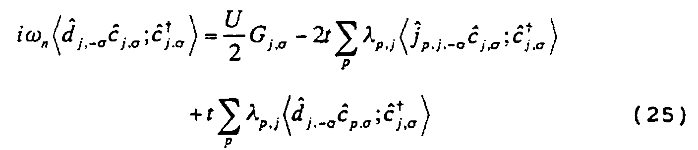
 The on-site Green function
 was introduced. To solve the equation, obtained, 〈d andj ,-σ c andj ,σ;c and † / j,σ〉 has to be analyzed. In case of half-filled models, this equation of motion is
 Here again, with reference to the Gros theory, approximation is introduced. It is the following translation.
 Here is assumed that there is no dependency on spin. That is, assuming
 becomes the density of states of the system. For later numerical calculation of densities of states, δ=0.0001 will be used.

 That is, spin-spin interaction exists only between nearest-neighbor sites. For the purpose of calculating spontaneous magnetization M at a finite temperature T, statistical mechanics of an equilibrium system is introduced. A partition function Z is defined as follows.
 where {Sp} in the symbol of the sum pertains to the sum regarding all spin states. Spontaneous magnetization is defined as the statistical average of spins as follows.
 where the expected value <Sp> is
 and n+1 is the total number of spins. M is generally a vector quantity in a spin space, but its absolute value M=|M| is calculated.
 A self-consistent equation ensuring spontaneous magnetization obtained by using a partition function by the simplified Hamiltonian becomes µp results in
 is obtained.
 Here is employed as the transfer tp,q,
 In this model, hopping is possible only between nearest-neighbor sites.
 Here,
Here, and the staircase function
 is calculated. The staircase function obtained is converted by a technique called "unfolding" such that the density of states becomes constant in average. By using quantum levels obtained in this manner, nearest-neighbor level spacing distribution P(s) and Δ3 statistics of Dyson and Metha are calculated as quantum level statistics. As taught in a literature ((36) L.E. Reich1, The transition to chaos: in conservative classical systems: quantum manifestations (Springer, New York, 1992) (37) F. Haake, Quantum Signatures of chaos, (Springer-Verlag, 1991)), by using these statistics, it can be detected whether quantum chaos has been generated or not. It is also known that a quantum chaotic system is sensitive to perturbation from outside similarly to the classical chaotic system, and analysis of quantum chaos is important as a polestar of designs of non-linear materials.

 Here is employed as the transfer tp,q,
 In this equation, p,q=-q,p is a random real number satisfying
 Here,
Here, and the staircase function
 is calculated. The staircase function obtained is converted by a technique called "unfolding" such that the density of states becomes constant in average. By using quantum levels obtained in this manner, nearest-neighbor level spacing distribution P(s) and Δ3 statistics of Dyson and Metha are calculated as quantum level statistics. As taught in a literature ((36) L.E. Reichl, The transition to chaos: in conservative classical systems: quantum manifestations (Springer, New York, 1992) (37) F. Haake, Quantum Signatures of chaos, (Springer-Verlag, 1991)), by using these statistics, it can be detected whether quantum chaos has been generated or not. It is also known that a quantum chaotic system is sensitive to perturbation from outside similarly to the classical chaotic system, and analysis of quantum chaos is important as a polestar of designs of non-linear materials.




 The on-site Green function
 is especially important.
 is obtained. Then, the approximation shown below is introduced, following Gros ((35) C. Gros, Phys. Rev. B50, 7295(1994)). If the site p is the nearest-neighbor site of the site j, the resolution
 was introduced. To solve the equation, obtained, 〈d andj ,-σ c andj ,σ;c and † / j,σ〉 has to be analyzed. In case of half-filled models, this equation of motion is
 Here again, with reference to the Gros theory, approximation is introduced. It is the following translation.
 Here is assumed that there is no dependency on spin. That is, assuming
 becomes the density of states of the system. For later numerical calculation of densities of states, δ=0.0001 will be used.

 That is, spin-spin interaction exists only between nearest-neighbor sites. For the purpose of calculating spontaneous magnetization M at a finite temperature T, statistical mechanics of an equilibrium system is introduced. A partition function Z is defined as follows.
 where {Sp} in the symbol of the sum pertains to the sum regarding all spin states. Spontaneous magnetization is defined as the statistical average of spins as follows.
 where the expected value <Sp> is
 and n+1 is the total number of spins. M is generally a vector quantity in a spin space, but its absolute value M=|M| is calculated.
 A self-consistent equation ensuring spontaneous magnetization obtained by using a partition function by the simplified Hamiltonian becomes µp results in

 was used. This function P2(s, ρ) coincides with P(s) of Poisson distribution under ρ=1, and coincides with P(s) of GOE distribution under ρ=0. That is, by changing ρ from 0 to 1, quantum level statistics from those of quantum chaotic systems to those of integrable systems can be interpolated. The Berry-Robnik parameter is the value of ρ obtained by optimum approximation of P(s) obtained by numerical calculation with P2(s, ρ) shown above. Within the range of semiclassical approximation, ρ is the ratio in volume of regular regions (integrable systems and regions capable of perturbing development therefrom) in a phase space.