EP1190278B1 - Method and hardware architecture for controlling a process or for processing data based on quantum soft computing - Google Patents

Abstract

A method of controlling a process (Plant) driven by a control signal (U*) for producing a corresponding output comprises producing an error signal (ε) as a function of a state of the process (X) and of a reference signal (Y), generating a control signal (U*) as a function of the error signal (ε) and of a parameter adjustment signal (CGS) and feeding it to the process (Plant), deriving a signal (S) representative of a quantity to be minimized calculated by processing paired values of the state (X) of the process and the control signal (U*), calculating a correction signal (K2) from a set of several different values of the control signal (U*), that minimize the derived signal (S) to be minimized, calculating the parameter adjustment signal (CGS) by a neural network and fuzzy logic processor from the error signal (ε) and correction signal (K2). The method of the invention is characterized in that the correction signal (K2) is periodically calculated by a Quantum Genetic Search Algorithm consisting in a merging of a genetic algorithm and a quantum search algorithm. A hardware embodiment of the method of the invention has been disclosed.

Description

FIELD OF THE INVENTION
• This invention generally relates to a method and a hardware for controlling a process or for processing data in a database, and more specifically to control a process and/or including search-of-minima intelligent operations.
• The method of the invention is outstandingly useful for minimum searching among a set of values and in particular for realizing hardware control systems exploiting artificial intelligence to robust smart control a nonlinear process and/or to search in a database.
BACKGROUND OF THE INVENTION
• Feedback control systems are widely used to maintain the output of a dynamic system at a desired value in spite of external disturbances that would displace it from the desired value. For example, a household space heating furnace, controlled by a thermostat, is an example of a feedback control system. The thermostat continuously measures the air temperature inside the house, and when the temperature falls below a desired minimum temperature the thermostat turns the furnace on. When the interior temperature reaches the desired minimum temperature, the thermostat turns the furnace off. The thermostat-fumace system maintains the household temperature at a substantially constant value in spite of external disturbances such as a drop in the outside temperature. Similar types of feedback controls are used in many applications.
• A central component in a feedback control system is a controlled object, a machine or a process that can be defined as a "plant", whose output variable is to be controlled. In the above example, the "plant" is the house, the output variable is the interior air temperature in the house and the disturbance is the flow of heat (dispersion) through the walls of the house. The plant is controlled by a control system. In the above example, the control system is the thermostat in combination with the furnace. The thermostat-furnace system uses simple on-off feedback control system to maintain the temperature of the house. In many control environments, such as motor shaft position or motor speed control systems, simple on-off feedback control is insufficient. More advanced control systems rely on combinations of proportional feedback control, integral feedback control, and derivative feedback control. A feedback control based on a sum of proportional, plus integral, plus derivative feedback, is often referred as a PID control.
• A PID control system is a linear control system that is based on a dynamic model of the plant. In classical control systems, a linear dynamic model is obtained in the form of dynamic equations, usually ordinary differential equations. The plant is assumed to be relatively linear, time invariant, and stable. However, many real-world plants are time varying, highly nonlinear, and unstable. For example, the dynamic model may contain parameters (e.g., masses, inductance, aerodynamics coefficients, etc.) which are either only approximately known or depend on a changing environment. If the parameter variation is small and the dynamic model is stable, then the PID controller may be satisfactory. However, if the parameter variation is large or if the dynamic model is unstable, then it is common to add adaptive or intelligent (AI) control functions to the PID control system.
• Al control systems use an optimizer, typically a nonlinear optimizer, to program the operation of the PID controller and thereby improve the overall operation of the control system.
• Classical advanced control theory is based on the assumption that near equilibrium points all controlled "plants" can be approximated as linear systems. Unfortunately, this assumption is rarely true in the real world. Most plants are highly nonlinear, and often do not have simple control algorithms. In order to meet these needs for a nonlinear control, systems have been developed that use soft computing concepts such as genetic algorithms (GA), fuzzy neural networks (FNN), fuzzy controllers and the like. By these techniques, the control system evolves (changes) in time to adapt itself to changes that may occur in the controlled "plant" and/or in the operating environment.
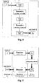
• A control system for controlling a plant based on soft computing is depicted in Fig. 1.
• Using a set of inputs, and a fitness function, the genetic algorithm works in a manner similar to an evolutional process to arrive at a solution which is, hopefully, optimal.
• The genetic algorithm generates sets of "chromosomes" (that is, possible solutions) and then sorts the chromosomes by evaluating each solution using the fitness function. The fitness function determines where each solution ranks on a fitness scale. Chromosomes (solutions) which are more fit, are those which correspond to solutions that rate high on the fitness scale. Chromosomes which are less fit, are those which correspond to solutions that rate low on the fitness scale.
• Chromosomes that are more fit are kept (survive) and chromosomes that are less fit are discarded (die). New chromosomes are created to replace the discarded chromosomes. The new chromosomes are created by crossing pieces of existing chromosomes and by introducing mutations.
• The PID controller has a linear transfer function and thus is based upon a linearized equation of motion for the controlled "plant". Prior art genetic algorithms used to program PID controllers typically use simple fitness and thus do not solve the problem of poor controllability typically seen in linearization models. As is the case with most optimizers, the success or failure of the optimization often ultimately depends on the selection of the performance (fitness) function.
• Evaluating the motion characteristics of a nonlinear plant is often difficult, in part due to the lack of a general analysis method. Conventionally, when controlling a plant with nonlinear motion characteristics, it is common to find certain equilibrium points of the plant and the motion characteristics of the plant are linearized in a vicinity near an equilibrium point. Control is then based on evaluating the pseudo (linearized) motion characteristics near the equilibrium point. This technique is scarcely, if at all, effective for plants described by models that are unstable or dissipative.
• Computation of optimal control based on soft computing includes GA as the first step of global search for optimal solution on a fixed space of positive solutions. The GA searches for a set of control weights for the plant. Firstly the weight vector K={k _l,...,k _n } is used by a conventional proportional-integral-differential (PID) in the generation of a signal δ(K) which is applied to the plant. The entropy
• S(δ(K)) associated to the behaviour of the plant on this signal is assumed as a fitness function to minimize. The GA is repeated several times at regular time intervals in order to produce a set of weight vectors. The vectors generated by GA are then provided to a FNN and the output of the FNN to a fuzzy controller. The output of the fuzzy controller is a collection of gain schedules for the PID - controller that controls the plant. For soft computing systems based on GA, there is very often no real control law in the classical control sense, but rather, control is based on a physical control law such as minimum entropy production.
• This allows robust control because the GA, combined with feedback, guarantee robustness. However, robust control is not necessarily optimal control. The GA attempts to find a global optimum solution for a given solution space. Any random disturbance (m(t) in Fig. 1) of the plant can "kick" the GA into a different solution space.
• It is desirable, however, to search for a global optimum in multiple solution spaces in order to find a "universal" optimum.
• The application of new knowledge-based control algorithms in advanced intelligent control theory of complex dynamic systems (as in controlling objects) has brought in necessity of the development of new processing methods such as Computational Intelligence (CI). Traditional computing basic tools for CI is GA, FNN, Fuzzy Sets theory, Evolution Programming, Qualitative Probabilistic Reasoning and etc. Application of CI in the advanced control theory of complex system motion has brought to two researching ways: 1) the study of stable non-equilibrium motion; and 2) an unstable non-equilibrium motion of complex dynamic systems.
• In the first case (of stable non-equilibrium motion) the development and design of intelligent control algorithms can be described in the structure submitted in Fig. 1.
• The peculiarity of the given structure is the consideration of the control object in accordance with the fuzzy system theory as a "black box" or non-linear models of plants. The study and optimization of "input-output" relations is based on soft computing as GA, FNN and fuzzy control (FC) for the description of the changing law of a PID-controller parameters with a minimum entropy production and control error. At the small random initial states, uncontrollable external excitations or small change of parameters or structure of controlled objects (plants), such an approach guarantees a robust and stable control for fixed spaces of possible excitations and solutions.
• In case of a global unstable dynamic control objective such an approach based on the presence of a robust and stable control does not guarantee success in principle. For such a kind of unstable dynamic control objectives, the development of new intelligent robust algorithms based on the knowledge about a movement of essentially non-linear unstable non-holonomic dynamic systems is necessary.
• The US patent No. 5,971,579, upon which the preamble of the independent claims is drafted, discloses a hardware unit and a method for determining gains of a PID (Proportional, Integral, Differential) controller using a genetic algorithm.
OBJECT AND SUMMARY OF THE INVENTION
• It has been found and is the object of the present invention a new method and a respective hardware architecture for controlling a generic process using an algorithm that is obtained substantially by merging a Genetic Algorithm and a Quantum Search Algorithm.
• The invention is concisely defined in the attached claims.
BRIEF DESCRIPTION OF THE DRAWINGS
• The particular aspects and advantages of the invention will become clearer through the following description of several important embodiments of the and by referring to the attached drawings, wherein:
• Figure 1 is a general structure of an Intelligent Control System based on Soft-Computing;
• Figure 2 is a general structure of an Intelligent Smart Control System, based on Quantum Soft-Computing;
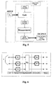
• Figure 3 is a block diagram of Quantum Algorithms;
• Figure 4 is a block diagram of an Encoder;
• Figure 5 is a general structure of the Quantum Block in Fig. 3;
• Figure 6 is an example of Quantum Circuit;
• Figure 7.a shows an example of tensor product transformation;
• Figure 7.b shows an example of dot product transformation;
• Figure 7.c shows the identity transformation;
• Figure 7.d shows an example of propagation rule;
• Figure 7.e shows an example of iteration rule;
• Figure 7.f explains the input/output tensor rule;
• Figure 8 is an example of a circuit realizing Grover's Quantum Gate;
• Figure 9 is a Grover's Quantum Gate;
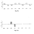
• Figure 10.a shows a possible set of input probability amplitudes;
• Figure 10.b shows a set of probability amplitudes after Step 1 of Fig. 8;
• Figure 10.c shows a set of probability amplitudes after Step 2 of Fig. 8;
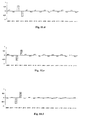
• Figure 10.d shows a set of probability amplitudes after Step 3 of Fig. 8;
• Figure 11.a is an example of a vector superposition;
• Figure 11.b is the set of vectors of Fig. 11.a after ⁴ H has been applied;
• Figure 11.c is the set of vectors of Fig. 11.b after the entanglement operator U _F (with x=001) has been applied;
• Figure 11.d is the set of vectors of Fig. 11.b after having applied the interference operator D _n ⊗I;
• Figure 11.e is the set of vectors of Fig. 11.b after having applied the entanglement operator U _F a second time;
• Figure 11.f is the set of vectors of Fig. 11.b after having applied the interference operator D _n ⊗I a second time;
• Table 1 resumes the information analysis of Grover's algorithm for a general number of iterations;
• Table 2 resumes the information analysis of Grover's algorithm for the first iteration;
• Table 3 resumes the information analysis of Grover's algorithm for the second iteration;
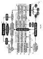
• Figure 12 shows the analogy between GA and QSA;
• Figure 13 is a block diagram for QGSA;
• Figure 14 is a block diagram of Quantum Genetic Search Algorithm;
• Figure 15 describes the structure of classical Genetic Algorithms and Quantum Searching Algorithms for global optimization;
• Figure 16 describes the general structure of Quantum Algorithms;
• Figure 17 depicts a quantum network for Quantum Searching Algorithm;
• Figure 18 is a diagram of a Quantum Searching Algorithm;
• Figure 19 shows several possible distributions of road profiles;
• Figure 20.a compares different dynamic behaviour of pitch angle of a vehicle after a simulation of a fuzzy control;
• Figure 20.b compares the phase portraits of the time diagrams of Fig. 20.a;
• Figure 21.a compares the entropy accumulation of the corresponding dynamic behaviour of Fig. 20.a;
• Figure 21.b compares the phase portraits of the time diagrams of Fig. 21.a;
DESCRIPTION OF SEVERAL EMBODIMENT OF THE INVENTION
• As stated above, the fundamental aspect of the present invention consists in the intuition that the merging of a Quantum Algorithm with a Genetic Algorithm obtaining what may be defined as a Quantum Genetic Search Algorithm would, as indeed has been found true, enhance formidably the function of teaching a Fuzzy Neural Network in implementing intelligent control systems as well as for searching data in a database.
• Such a merging has been possible because of the "similarity" between a Quantum Algorithm and a Genetic Algorithm, and in order to make more easily comprehensible the description of the novel Quantum Genetic Search Algorithm of the invention, it is deemed useful to preliminarily present a brief review of the Genetic Algorithm theory and of the Quantum Algorithm theory.
GENETIC ALGORITHMS
• Genetic Algorithms (GA's) are global search algorithms based on the mechanics of natural genetics and natural selection. In the genetic search, a finite length binary string represents each design variable and the set of all possible solutions is so encoded into a population of binary strings. Genetic transformations, analogous to biological reproduction and evolution, are subsequently used to vary and improve the encoded solutions. Usually, three main operators i.e. crossover, mutation and selection are used in the genetic search.
• The selection process is one that biases the search toward producing more fit members in the population and eliminating the less fit ones. Hence, a fitness value is first assigned to each string in the population. One simple approach to select members from an initial population is to assign each member a probability of being selected, on the basis of its fitness value. A new population pool of the same size as the original is then created with a higher average fitness value.
• The process of selection simply results in more copies of the dominant design to be present in the population. The crossover process allows for an exchange of design characteristics among members of the population pool with the intent of improving the fitness of the next generation. Crossover is executed by selecting strings of two mating parents, randomly choosing two sites on the strings, and swapping strings of 0's and 1's between these chosen sites.
• Mutation safeguards the genetic search process from a premature loss of valuable genetic material during selection and crossover. The process of mutation consists into choosing a few members from the population pool on the basis of their probability of mutation and switch 0 to 1 or vice versa at a randomly selected mutation rate on the selected string.
• In the foregoing discussion, the mechanics of the genetic search are simple. However, there are some key differences from traditional methods that contribute to the strength of the approach. GA's work on function evaluations alone and do not require function derivatives. While derivatives contribute to a faster convergence towards the optimum, they may also direct the search towards a local optimum. Furthermore, since the search proceeds from several points in the design space to another set of design points, the method has a higher probability of locating a global minimum as opposed to those schemes that proceed from one point to another. In addition, genetic algorithms work on a coding of design variables rather than variables themselves. This allows for an extension of these algorithms to design space consisting of a mix of continuous, discrete and integer variables.
• In the context of GAs operating on binary strings, a schema (or similarity template) is a string of symbols taken from the alphabet {0,1,#}. The character # is interpreted as "don't care" symbol, so that a schema can represent several bit strings. For example, the schema #10#1 represents four strings: 10011,01011,11001, and 11011. The number of non-# symbols is called the order O(H) of a schema H. The distance between the furthest two non-# symbols is called the defining length L(H) of the schema.
• Holland obtained a result (the schema theorem) that predicts how the number of strings in a population matching (or belonging to) a schema is expected to vary from one generation to the next (Holland, 1992). The theorem is as follows: $$E\left[m\left(H,t+1\right)\right]\ge m\left(H,t\right)\cdot \underset{\mathit{Selection}}{\underbrace{\frac{f\left(H,t\right)}{\bar{f}\left(t\right)}}}\cdot \underset{\mathit{Mutation}}{\underbrace{{\left(1-p_m\right)}^{\mathrm{O}\left(H\right)}}}\cdot \underset{\mathit{Crossover}}{\underbrace{\left[1-\stackrel{P_d\left(H,t\right)}{\overbrace{p_c\frac{L\left(H\right)}{N-1}\left(1-\frac{m\left(H,t\right)f\left(H,t\right)}{M\bar{f}\left(t\right)}\right)}}\right]}}$$

  

  where m(H,t) is the number of strings matching the schema H at generation t, ƒ(H,t) is the mean fitness of the strings matching H, ƒ̅(t) is the mean fitness of the strings in the population, p _m is the probability of mutation per bit, p _c is the probability of crossover, N is the number of bits in the strings, M is the number of strings in the population, and E[m(H,t + 1)] is the expected number of strings matching the schema H at generation t +1. This is slightly different version of Holland's original theorem. Equation (1) applies when crossover is performed taking both parents from the mating pool (Goldberg, 1989). The three horizontal curly brackets beneath the equation indicate which operators are responsible for each term. The bracket above the equation represents the probability of disruption of the schema H at generation t due to crossover P _d (H,t). Such a probability depends on the frequency of the schema in the mating pool but also on the intrinsic fragility of the schema L(H)/(N-1).
QUANTUM ALGORITHMS
• The problems solved by the quantum algorithms may be stated as follows:

  Input	A function ƒ:{0,1}n→{0,1}m
  Problem	Find a certain property of ƒ

• The structure of a quantum algorithm is outlined, by a high level representation, in the schematic diagram of Fig. 3.
• The input of a quantum algorithm is always a function ƒ from binary strings into binary strings. This function is represented as a map table, defining for every string its image. Function ƒ is firstly encoded into a unitary matrix operator U _F depending on ƒ properties. In some sense, this operator calculates ƒ when its input and output strings are encoded into canonical basis vectors of a Complex Hilbert Space: U _F maps the vector code of every string into the vector code of its image by ƒ.

  BOX 1: UNITARY MATRIX U F
  A squared matrix U F on the complex field is unitary if its inverse matrix coincides with its conjugate transpose:
  U F -1 =U F ↑
  A unitary matrix is always reversible and preserves the norm of vectors.

• When the matrix operator U _F has been generated, it is embedded into a quantum gate G, a unitary matrix whose structure depends on the form of matrix U _F and on the problem we want to solve. The quantum gate is the heart of a quantum algorithm. In every quantum algorithm, the quantum gate acts on an initial canonical basis vector (we can always choose the same vector) in order to generate a complex linear combination (let's call it superposition) of basis vectors as output. This superposition contains all the information to answer the initial problem.
• After this superposition has been created, measurement takes place in order to extract this information. In quantum mechanics, measurement is a non-deterministic operation that produces as output only one of the basis vectors in the entering superposition. The probability of every basis vector of being the output of measurement depends on its complex coefficient (probability amplitude) in the entering complex linear combination.
• The segmental action of the quantum gate and of measurement constitutes the quantum block. The quantum block is repeated k times in order to produce a collection of k basis vectors. Being measurement a non-deterministic operation, these basic vectors won't be necessarily identical and each one of them will encode a peace of the information needed to solve the problem.
• The last part of the algorithm consists into the interpretation of the collected basis vectors in order to get the right answer for the initial problem with a certain probability.
Encoder
• The behaviour of the encoder block is described in the detailed schematic diagram of Fig. 4.
• Function f is encoded into matrix U _F in three steps.
Step 1
• The map table of function ƒ:{0,1} ⁿ →{0,1} ^m is transformed into the map table of the injective function F:{0,1} ^n+m →{0,1} ^n+m such that: $$F\left(x_0,\dots ,x_{n-1},{\mathrm{<figure-callout\; id="0"\; label="y"\; filenames="imgf0007.png,imgf0010.png"\; state="\{\{state\}\}">y</figure-callout>}}_0,\dots ,y_{m-1}\right)=\left(x_0,\dots ,x_{n-1},f\left(x_0,\dots ,x_{n-1}\right)\oplus \left({\mathrm{<figure-callout\; id="0"\; label="y"\; filenames="imgf0007.png,imgf0010.png"\; state="\{\{state\}\}">y</figure-callout>}}_0,\dots ,y_{m-1}\right)\right)$$

  
• The need to deal with an injective function comes from the requirement that U _F is unitary. A unitary operator is reversible, so it can't map 2 different inputs in the same output. Since U _F will be the matrix representation of F, F is supposed to be injective. If we directly employed the matrix representation of function ƒ, we could obtain a non-unitary matrix, since ƒ could be non-injective. So, injectivity is fulfilled by increasing the number of bits and considering function F instead of function ƒ. Anyway, function ƒ can always be calculated from F by putting (y ₀, ..., y _m-1)=(0,..,0) in the input string and reading the last m values of the output string.

  BOX 2: XOR OPERATOR ⊕
  The XOR operator between two binary strings p and q of length m is a string s of length m such that the i-th digit of s is calculated as the exclusive OR between the i-th digits of p and q:
  p=(p 0, .., p n-1)
  q=(q 0, ..,q n-1)
  s = p ⊕ q = ((P 0+q 0) mod 2, .., (P n-1+q n-1) mod 2))

Step 2
• Function F map table is transformed into U _F map table, following the following constraint: $$\forall s\in {\left\{0,1\right\}}^{n+m}:U_F\left[\tau \left(s\right)\right]=\tau \left[F\left(s\right)\right]$$

  
• The code map τ : {0,1} ^n+m → C 2 ^n+m (C 2 ^n+m is the target Complex Hilbert Space) is such that: $$\tau \left(0\right)=\left(\begin{array}{c}1\\ 0\end{array}\right)=|0\rangle \mathrm{\hspace{0.17em}\hspace{1em}\tau }\left(1\right)=\left(\begin{array}{c}0\\ 1\end{array}\right)=|1\rangle$$

  

  $$\tau \left(x_0,\dots ,x_{n+m-1}\right)=\tau \left(x_0\right)\otimes \dots \otimes \tau \left(x_{n+m-1}\right)=|x_0\dots x_{n+m-1}\rangle$$

  
• Code τ maps bit values into complex vectors of dimension 2 belonging to the canonical basis of C ². Besides, using tensor product, τ maps the general state of a binary string of dimension n into a vector of dimension 2 ⁿ , reducing this state to the joint state of the n bits composing the register. Every bit state is transformed into the corresponding 2-dimesional basis vector and then the string state is mapped into the corresponding 2 ⁿ -dimesional basis vector by composing all bit-vectors through tensor product. In this sense tensor product is the vector counterpart of state conjunction.

  BOX 3: VECTOR TENSOR PRODUCT ⊗
  The tensor product between two vectors of dimensions h and k is a tensor product of dimension h·k, such that: product of dimension h·k, such that:
  $|x\rangle \otimes |y\rangle =\left(\begin{array}{c}{x}_1\\ \dots \\ x_h\end{array}\right)\otimes \left(\begin{array}{c}{\mathrm{<figure-callout\; id="1"\; label="y"\; filenames="imgf0003.png,imgf0004.png"\; state="\{\{state\}\}">y</figure-callout>}}_1\\ \dots \\ y_k\end{array}\right)=\left(\begin{array}{c}{x}_1{\mathrm{<figure-callout\; id="1"\; label="y"\; filenames="imgf0003.png,imgf0004.png"\; state="\{\{state\}\}">y</figure-callout>}}_1\\ \dots \\ x_1{y}_k\\ \dots \\ x_{\mathrm{<figure-callout\; id="1"\; label="h\; y"\; filenames="imgf0003.png,imgf0004.png"\; state="\{\{state\}\}">h</figure-callout>}}{y}_{}{}_1\\ \dots \\ x_h{y}_k\end{array}\right)\Rightarrow$

Examples: Vector Tensor Products

• $\left(0,0\right)\stackrel{\tau }{\to }\left(\begin{array}{c}1\\ 0\end{array}\right)\otimes \left(\begin{array}{c}1\\ 0\end{array}\right)=\left(\begin{array}{c}1\\ 0\\ 0\\ 0\end{array}\right)=|00\rangle$	$\left(0,1\right)\stackrel{\tau }{\to }\left(\begin{array}{c}1\\ 0\end{array}\right)\otimes \left(\begin{array}{c}0\\ 1\end{array}\right)=\left(\begin{array}{c}0\\ 1\\ 0\\ 0\end{array}\right)=|01\rangle$
  $\left(1,0\right)\stackrel{\tau }{\to }\left(\begin{array}{c}0\\ 1\end{array}\right)\otimes \left(\begin{array}{c}1\\ 0\end{array}\right)=\left(\begin{array}{c}0\\ 0\\ 1\\ 0\end{array}\right)=|10\rangle$	$\left(1,1\right)\stackrel{\tau }{\to }\left(\begin{array}{c}0\\ 1\end{array}\right)\otimes \left(\begin{array}{c}0\\ 1\end{array}\right)=\left(\begin{array}{c}0\\ 0\\ 0\\ 1\end{array}\right)=|11\rangle$

• Basis vectors are denoted using the ket notation |i>. This notation is taken from Dirac description of quantum mechanics.
Step 3
• U _F map table is transformed into U _F using the following transformation rule: $${\left[U_F\right]}_{ij}=1\iff U_F|j\rangle =|i\rangle$$

  
• This rule can easily be understood considering vectors |i> and |j> as column vectors. Belonging these vectors to the canonical basis, U _F defines a permutation map of the identity matrix rows. In general, row |j> is mapped into row |i>.
• This rule will be illustrated in detail on the first example of quantum algorithm: Grover's algorithm.
Quantum block
• The heart of the quantum block is the quantum gate, which depends on the properties of matrix U _F . The scheme in Fig. 5 gives a more detailed description of the quantum block.
• The matrix operator U _F in Fig. 5 is the output of the encoder block represented in Fig. 4. Here, it becomes the input for the quantum block.
• This matrix operator is firstly embedded into a more complex gate: the quantum gate G. Unitary matrix G is applied k times to an initial canonical basis vector |i> of dimension 2 ^n+m . Every time, the resulting complex superposition G|0..01..1> of basis vectors is measured, producing one basis vector lx _i > as result. All the measured basis vectors {|x _l >....,|x _k >} are collected together. This collection is the output of the quantum block.
• The "intelligence" of such algorithms is in the ability to build a quantum gate that is able to extract the information necessary to find the required property of ƒ and to store it into the output vector collection.
• The structure of the quantum gate for every quantum algorithm will be discussed in detail, observing that a general description is possible.
• In order to represent quantum gates we are going to employ some special diagrams called quantum circuits.
• An example of quantum circuit is reported in Fig. 6. Every rectangle is associated to a matrix 2 ⁿ ×2 ⁿ , where n is the number of lines entering and leaving the rectangle. For example, the rectangle marked U _F is associated to matrix U _F .
• Quantum circuits let us give a high-level description of the gate and, using some transformation rules, which are listed in Fig. 7, it is possible to compile them into the corresponding gate-matrix.
• It will be clearer how to use these rules when we afford the first examples of quantum algorithm.

  BOX 4: MATRIX TENSOR PRODUCT ⊗
  The tensor product between two matrices X n×m and Y h×k is a (block) matrix (n·h)×(m·k) such that:
  $X=\left[\begin{array}{ccc}{x}_{11}& \dots & x_{1m}\\ \dots & \dots & \dots \\ x_{\mathrm{<figure-callout\; id="1"\; label="n"\; filenames="imgf0003.png,imgf0004.png"\; state="\{\{state\}\}">n</figure-callout>}1}& \dots & x_{nm}\end{array}\right]$ with $X\otimes Y=\left[\begin{array}{ccc}{x}_{11}Y& \dots & x_{1m}Y\\ \dots & \dots & \dots \\ x_{n1}Y& \dots & x_{nm}Y\end{array}\right]$

Example: Matrix Tensor Product
• $$\left[\begin{array}{cc}1& 2\\ 3& 4\end{array}\right]\otimes \left[\begin{array}{cc}5& 6\\ 7& 8\end{array}\right]=\left[\begin{array}{cc}1\cdot \left[\begin{array}{cc}5& 6\\ 7& 8\end{array}\right]& 2\cdot \left[\begin{array}{cc}5& 6\\ 7& 8\end{array}\right]\\ 3\cdot \left[\begin{array}{cc}5& 6\\ 7& 8\end{array}\right]& 4\cdot \left[\begin{array}{cc}5& 6\\ 7& 8\end{array}\right]\end{array}\right]=\left[\begin{array}{cccc}5& 6& 10& 12\\ 7& 8& 14& 16\\ 15& 18& 20& 24\\ 21& 24& 28& 32\end{array}\right]$$

  
Decoder
• The decoder block has the function to interpret the basis vectors collected after the iterated execution of the quantum block. Decoding these vectors means to retranslate them into binary strings and interpreting them directly if they already contain the answer to the starting problem or use them, for instance as coefficients vectors for some equation system, in order to get the searched solution. This part will not being investigated in detail because it is a non-interesting easy classical part.
• Because of the particular importance of the Grover's Algorithm in the realization of controllers, a brief description of the Grover's algorithm is given.
GROVER'S PROBLEM
• Grover's problem is so stated:

  Input	A function ƒ:{0,1} n →{0,1} such that
  	∃x∈{0,1} n : (ƒ(x)=1∧∀y∈{0,1} n :x≠y⇒ƒ(y)=0)
  Problem	Find x

• In Deutsch-Jozsa's algorithm we distinguished two classes of input functions and we were supposed to decide what class the input function belonged to. In this case the problem is in some sense identical in its form, even if it is harder because now we are dealing with 2 ⁿ classes of input functions (each function of the kind described constitutes a class).
Encoder
• In order to make the discussion more comprehensible, we prefer firstly to consider a special function with n=2. Then we discuss the general case with n=2 and finally we analyze the general case with n>0.
A1. Introductory example
• Let's consider the case: $$n=2\mathrm{\hspace{1em}\hspace{0.17em}}f\left(01\right)=1$$

  
• In this case ƒ map table is so defined:

  x	ƒ(x)
  00	0
  01	1
  10	0
  11	0

Step 1
• Function ƒ is encoded into injective function F, built according to the usual statement: $$F:{\left\{0,1\right\}}^{n+1}\to {\left\{0,1\right\}}^{n+1}:F\left(x_0,x_1,y_0\right)=\left(x_0,x_1,f\left(x_0,x_1\right)\oplus y_0\right)$$

  
• Then F map table is:

  (x 0,x 1,y 0)	F(x 0,x 1,y 0)
  000	000
  010	011
  100	100
  110	110
  001	001
  011	010
  101	101
  111	111

Step 2
• Let's now encode F into the map table of U _F using the usual rule: $$\forall s\in {\left\{0,1\right\}}^{n+1}:U_F\left[\tau \left(s\right)\right]=\tau \left[F\left(s\right)\right]$$

  

  where τ is the code map defined in Equation (3). This means:

  |x 0 x 1 y 0>	U F |x 0 x 1 y 0 >
  |000>	|000>
  |010>	|011>
  |100>	|100>
  |110>	|110>
  |001>	|001>
  |011>	|011>
  |101>	|101>
  |111>	|111>

Step 3
• From the map table of U _F we are supposed to calculate the corresponding matrix operator.
• This matrix is obtained from Equation (4) using the rule: $${\left[U_F\right]}_{ij}=1\iff U_F|j\rangle =|i\rangle$$

  

  U _F is so calculated:

  U F	|00>	|01>	|10>	|11>
  |00>	I	0	0	0
  |01>	0	C	0	0
  |10>	0	0	I	0
  |11>	0	0	0	I

• The effect of this matrix is to leave unchanged the first and the second input basis vectors of the input tensor product, flipping the third one when the first vector is |0> and the second is |1>. This agrees with the constraints on U _F stated above.
B. General case with n=2
• Let's now take into consideration the more general case: $$n=2\mathrm{\hspace{1em}\hspace{1em}\hspace{0.17em}}f\left(\underset{‾}{x}\right)=1$$

  
• The corresponding matrix operator is:

  U F	|00>	|01>	|10>	|11>
  |00>	M 00	0	0	0
  |01>	0	M 01	0	0
  |10>	0	0	M 10	0
  |11>	0	0	0	M 11

  with M _x =C∧∀i≠x:M _t =I.
C. General case
• It is fairly natural to generalize operator U _F from the case n=2 to the case n>1. In fact, we always find operator C on the main diagonal of the block matrix, in correspondence of the celled labeled by vector | x >, where x is the binary string having image one by ƒ. Therefore:

  U F	|00>	|01>	...	|11>
  |00>	M 00	0	...	0
  |01>	0	M 01	...	0
  ...	...	...	...	...
  |11>	0	0	...	M 11

  with M _x =C∧∀Ci≠x:M ₁ =I.
• Matrix U _F , the output of the encoder, is embedded into the quantum gate. We describe this gate using a quantum circuit such that depicted in Fig. 8.
• Operator D _n is called diffusion matrix of order n and it is responsible of interference in this algorithm. It plays the same role as QFT _n in Shor's algorithm and of ⁿ H in Deutsch-Jozsa's and Simon's algorithms. This matrix is defined in this way:

  D n	|0..0>	|0..1>	...	|i>	...	|1..0>	|1..1>
  |0..0>	-1+1/2 n-1	1/2 n-1	...	1/2 n-1	...	1/2 n-1	1/2 n-1
  |0..1>	1/2 n-1	-1+1/2 n-1	...	1/2 n-1	...	1/2 n-1	1/2 n-1
  |i>	1/2 n-1	1/2 n-1	...	-1+1/2 n-1	...	1/2 n-1	1/2 n-1
  |1..0>	1/2 n-1	1/2 n-1	...	1/2 n-1	...	-1+1/2 n-1	1/2 n-1
  |1..1>	1/2 n-1	1/2 n-1	...	1/2 n-1	...	1/2 n-1	-1+1/2 n-1

• Using the identity transformation (Fig. 7.c), the previous circuit can be compiled into the circuit of Fig. 9.
A2. Introductory example: Dynamic Analysis
• In the introductory example we dealt above, U _F had the following form:

  U F	|00>	|01>	|10>	|11>
  |00>	I	0	0	0
  |01>	0	C	0	0
  |10>	0	0	I	0
  |11>	0	0	0	I

• Let's calculate the quantum gate G=[(D ₂⊗I) ·U _F ] ^h ·(²⁺¹ H) in this case:

  3 H	|00>	|01>	|10>	|11>
  |00>	H/2	H/2	H/2	H/2
  |01>	H/2	-H/2	H/2	-H/2
  |10>	H/2	H/2	-H/2	-H/2
  |11>	H/2	-H/2	-H/2	H/2

  D 2 ⊗I	|00>	|01>	|10>	|11>
  |00>	-I/2	1/2	I/2	I/2
  |01>	I/2	-I/2	I/2	I/2
  |10>	I/2	I/2	-I/2	I/2
  |11>	1/2	1/2	1/2	-I/2

  U F . 3 H	|00>	|01>	|10>	|11>
  |00>	H/2	H/2	H/2	H/2
  |01>	CH/2	-CH/2	CH/2	-CH/2
  |10>	H/2	H/2	-H/2	-H/2
  |11>	H/2	-H/2	-H/2	H/2

• Choosing h=1, we obtain:

  G	|00>	|01>	|10>	|11>
  |00>	(C+I)H/4	(-C-I)H/4	(C-3I)H/4	(-C-I)H/4
  |01>	(-C+3I)H/4	(C+I)H/4	(-C-I)H/4	(C+I)H/4
  |10>	(C+I)H/4	(-C-I)H/4	(C+I)H/4	(-C+3I)H/4
  |11>	(C+I)H/4	(-C+3I)H/4	(C+I)H/4	(-C-I)H/4

• Now, consider the application of G to vector |001>: $$G|001\rangle =\frac{1}{4}|00\rangle \otimes \left(C+I\right)H|1\rangle +\frac{1}{4}|01\rangle \otimes \left(-C+3I\right)H|1\rangle +\frac{1}{4}|10\rangle \otimes \left(C+I\right)H|1\rangle +\frac{1}{4}|11\rangle \otimes \left(C+I\right)H|1\rangle$$

  
• Let's calculate the operator (-C+3I)H/4. Then

  -C+3I	|0>	|1>
  |0>	3	-1
  |1>	-1	3

  (-C+3I)H/4	|0>	|1>
  |0>	1/23/2	1/21/2
  |1>	1/23/2	-1/21/2

• Therefore: $$\frac{1}{4}\left(-C+3I\right)H|1\rangle =\frac{1}{\sqrt{2}}\left(|0\rangle -|1\rangle \right)$$

  
• Let's calculate the operator (C+I)H/4. Then:

  C+I	|0>	|1>
  |0>	1	1
  |1>	1	1

  (C+I)H/4	|0>	|1>
  |0>	1/23/2	0
  |1>	1/23/2	0

• Therefore: $$\frac{1}{4}\left(C+I\right)H|1\rangle =0$$

  
• This means that |001> is mapped into vector |01>(|0>-|1>)/2^1/2. Taking the binary values of the first two vectors of dimension 2, we find x.
• It might be useful to picture the evolution of the probability amplitude of every basis vector while operator ³ H. U _F and D ₂ ⊗I are applied in sequence. This is done in Fig. 10.
• Operator ³ H puts the initial canonical basis vector |001> into a superposition of all basis vectors with the same (real) coefficients in modulus, but with positive sign if the last vector is |0>, negative otherwise. Operator U _F creates correlation: it flips the third vector if the first two vector are |0> and |1>. Finally, D ₂⊗l produces interference: for every basis vector | x ₀ x ₁ y ₀> it calculates its output probability amplitude α' _x0x1y0 by inverting its initial probability amplitude α _x0x1y0 and summing the double of the mean α _y0 of the probability amplitude of all vectors in the form |x ₀ x ₁ y ₀>. In our example α ₀=1/(4.2^1/2), α ₁= -1/(4.2^1/2). Take, for instance, basis vector |000>. Then α'₀₀₀=-α₀₀₀+2α ₀=-1/(2·2^1/2)+2/(4·2^1/2)=0.
D. General case with n=2
• In general, if n=2, U _F has the following form:

  U F	|00>	|01>	|10>	|11>
  |00>	M 00	0	0	0
  |01>	0	M 01	0	0
  |10>	0	0	M 10	0
  |11>	0	0	0	M 11

  where M _x = C∧∀i≠ x :M _i =I ( x,i∈:{0,1} ⁿ ).
• Let's calculate the quantum gate G=(D ₂ ⊗I)·U _F ·(²⁺¹ H) in this general case:

  
• Now, consider the application of G to vector |001>: $$G|001\rangle =\frac{1}{4}|00\rangle \otimes \left(-M_{00}+{\mathrm{<figure-callout\; id="01"\; label="M"\; filenames="imgf0006.png"\; state="\{\{state\}\}">M</figure-callout>}}_{01}+{\mathrm{<figure-callout\; id="10"\; label="M"\; filenames="imgf0003.png,imgf0006.png"\; state="\{\{state\}\}">M</figure-callout>}}_{10}+M_{11}\right)H|1\rangle +\frac{1}{4}|01\rangle \otimes \left(M_{00}-M_{01}+{\mathrm{<figure-callout\; id="10"\; label="M"\; filenames="imgf0003.png,imgf0006.png"\; state="\{\{state\}\}">M</figure-callout>}}_{10}+M_{11}\right)H|1\rangle +\frac{1}{4}|10\rangle \otimes \left(M_{00}+{\mathrm{<figure-callout\; id="01"\; label="M"\; filenames="imgf0006.png"\; state="\{\{state\}\}">M</figure-callout>}}_{01}-M_{10}+M_{11}\right)H|1\rangle +\frac{1}{4}|11\rangle \otimes \left(M_{00}+{\mathrm{<figure-callout\; id="01"\; label="M"\; filenames="imgf0006.png"\; state="\{\{state\}\}">M</figure-callout>}}_{01}+{\mathrm{<figure-callout\; id="10"\; label="M"\; filenames="imgf0003.png,imgf0006.png"\; state="\{\{state\}\}">M</figure-callout>}}_{10}-M_{11}\right)H|1\rangle$$

  
• Consider the following cases:
  x =00: $$G|001\rangle =\frac{1}{4}|00\rangle \otimes \left(-C+3I\right)H|1\rangle +\frac{1}{4}|01\rangle \otimes \left(C+I\right)H|1\rangle +\frac{1}{4}|10\rangle \otimes \left(C+I\right)H|1\rangle +\frac{1}{4}|11\rangle \otimes \left(C+I\right)H|1\rangle =|00\rangle \left(\frac{|0\rangle -|1\rangle }{\sqrt{2}}\right)$$

  

  $$\begin{array}{l}\underset{‾}{x}=01:\\ G|001\rangle =\frac{1}{4}|00\rangle \otimes \left(C+I\right)H|1\rangle +\frac{1}{4}|01\rangle \otimes \left(-C+3I\right)H|1\rangle +\frac{1}{4}|10\rangle \otimes \left(C+I\right)H|1\rangle +\frac{1}{4}|11\rangle \otimes \left(C+I\right)H|1\rangle =|01\rangle \left(\frac{|0\rangle -|1\rangle }{\sqrt{2}}\right)\end{array}$$

  

  $$\begin{array}{l}\underset{‾}{x}=10:\\ G|001\rangle =\frac{1}{4}|00\rangle \otimes \left(C+I\right)H|1\rangle +\frac{1}{4}|01\rangle \otimes \left(C+I\right)H|1\rangle +\frac{1}{4}|10\rangle \otimes \left(-C+3I\right)H|1\rangle +\frac{1}{4}|11\rangle \otimes \left(C+I\right)H|1\rangle =|10\rangle \left(\frac{|0\rangle -|1\rangle }{\sqrt{2}}\right)\end{array}$$

  

  $$\begin{array}{l}\underset{‾}{x}=11:\\ G|001\rangle =\frac{1}{4}|00\rangle \otimes \left(C+I\right)H|1\rangle +\frac{1}{4}|01\rangle \otimes \left(C+I\right)H|1\rangle +\frac{1}{4}|10\rangle \otimes \left(C+I\right)H|1\rangle +\frac{1}{4}|11\rangle \otimes \left(-C+3I\right)H|1\rangle =|11\rangle \left(\frac{|0\rangle -|1\rangle }{\sqrt{2}}\right)\end{array}$$

  
• This means that if we measure the output vector and encode back the first two basis vectors of dimension 2 in the resulting tensor product, we get the following results:

  x	Result	Probability
  00	00	1
  01	01	1
  10	10	1
  11	11	1

E. General case (n>0)
• In the general case n>0, U _F has the following form:

  U F	|0..0>	|0..1>	...	|1..1>
  |0..0>	M 0..0	0	0	0
  |0..1>	0	M 0..1	0	0
  ...	...	...	...	...
  |1..1>	0	0	0	M 1..1

  where M _x =C∧1∀i≠ x :M ₁ =1( x ,i∈:{0,1} ⁿ ).
• Let's calculate the quantum gate G=[(D_n⊗I)·V_F]^h·(ⁿ⁺¹H)

  n+1 H	|0..0>	...	| j >	...	|1..1>
  |0..0>	H/2 n/2	...	H/2 n/2	...	H/2 n/2
  ...	...	...	...	...	... ...
  |i>	H/2 n/2	...	(-1) i·j H/2 n/2	...	(-1) i·(i..j) H/2 n/2
  ...	...	...	...	...	...
  |11>	H/2 n/2	...	(-1)(1..1)·j H/2 n/2	...	(-1)(1..1)
  					(1..1) H/2 n/2

  D n ⊗I	|0..0>	|0..1>	...	|i>	...	|1..0>	|1..1>
  |0..0>	-I+I/2 n-1	I/2n-1	...	I/2n-1	...	I/2n-1	I/2n-1
  |0..1>	I/2n-1	-I+I/2 n-1	...	I/2n-1	...	I/2n-1	I/2n-1
  ...	...	...	...	...	...	...	...
  |i>	I/2n-1	I/2n-1	...	-I+I/2n-1	...	I/2n-1	I/2n-1
  ...	...	...	...	...	...	...	...
  |1..0>	I/2n-1	I/2n-1	...	I/2n-1	...	-I+I/2 n-1	I/2n-1
  |1..1>	I/2n-1	I/2n-1	...	I/2n-1	...	I/2n-1	-I+I/2 n-1

  U F . n+1 H	|0..0>	...	|j>	...	|1..1>
  |0..0>	M 0..0 H/2 n/2	...	M 0..0 H/2 n/2	...	M 0..0 H/2 n/2
  ...	...	...	...	...	...
  |i>	M i H/2 n/2	...	(-1)i·j M i H/2 n/2	...	(-1)i·(1..1) M i H/2 n/2
  ...	...	...	...	...	...
  |1..1>	M 1..1 H/2 n/2	...	(-1)(1..1)-j M 1..1 H/2 n/2	...	(-1)(1..1)·(1..1) M 1..1 H/2 n/2

• Now, suppose h=1. Then:

  G h=1	|0..0>	...
  |0..0>	(-M 0..0 +Σ j∈(0,1) nM i /2 n-1 )H/2 n/2	...
  ...	...	...
  |i>	(-M i +Σ j∈(0,1) n M i /2 n-l )H/2 n/2	...
  ...	...	...
  |1..1>	(-M 1..1+Σ j∈(0,1) n M i /2 n-1 )H/2 n/2	...

• Being M _x =C and ∀i≠ x :M _i = I, this column may be written as:

  G h=l	|0..0>	...
  |0..0>	(-I+Σ j∈{0,1}n-{ x } I/2 n-1 + C/2 n-1 )H/2 n/2	...
  | x >	(-C+Σ j∈{0,1}n-{ x } I/2 n-1 +C/2 n-1 )H/2 n/2	...
  |1..1>	(-I+Σ j∈{0,1}n-{ x } I/2 n-1 +C/2 n-1 )H/2 n/2	...

  and so:

  G h=1	|0..0>	...
  |0..0>	{[-1+(2 n -1)/2 n-1]1+C/2 n-1}H/2 n/2	...
  ...	...	...
  | x >	{(2 n -1)/2 n-1 1+[-1+1/2 n-1]C}H/2 n/2	...
  ...	...	...
  |1..1>	{[-1+(2 n -1)/2 n-1]I+C/2 n-1}H/2 n/2	...

• Now, consider to apply matrix operator {[-1+(2 ⁿ -1)/2 ^n-1]I+ C/2 ^n-1}H/2 ^n/2 and matrix operator {(2 ⁿ -1)/2 ^n-1 I+ [-1+1/2 ^n-1]C}H/2 ^n/2 to vector |1>: $$\frac{1}{2^{n/2}}\left\{\left[-1+\frac{2^n-1}{2^{n-1}}\right]I+\frac{1}{2^{n-1}}C\right\}H|1\rangle =\left(-1+\frac{2^n-2}{2^{n-1}}\right)\frac{|0\rangle -|1\rangle }{2^{\frac{\left(n+1\right)}{2}}}$$

  

  $$\frac{1}{2^{n/2}}\left\{\frac{2^n-1}{2^{n-1}}I+\left[-1+\frac{1}{2^{n-1}}\right]C\right\}H|1\rangle =\left(+1+\frac{2^n-2}{2^{n-1}}\right)\frac{|0\rangle -|1\rangle }{2^{\frac{\left(n+1\right)}{2}}}$$

  
• This means: $$G_{h=1}|0\dots 01\rangle =\left[\left(-1+\frac{2^n-2}{2^{n-1}}\right)|0\dots 0\rangle +\left(-1+\frac{2^n-2}{2^{n-1}}\right)|0\dots 1\rangle +\dots +\left(+1+\frac{2^n-2}{2^{n-1}}\right)|\underset{‾}{x}\rangle +\dots +\left(-1+\frac{2^n-2}{2^{n-1}}\right)|1\dots 1\rangle \right]\otimes \frac{|0\rangle -|1\rangle }{2^{\frac{\left(n+1\right)}{2}}}$$

  

  which can be written as a block vector:

  G h=1 |0..01>
  |0..0>	[-1+(2 n -2)/2 n-1]/2 n/2 H|1>
  ...	...
  | x>	[+1+(2 n -2)/2 n-1]/2 n/2 H|1>
  ...	...
  |1..1>	[-1+(2 n -2)/2 n-1]/2 n/2 H|1>

• Now, let us suppose of applying the operator (D _n ⊗I) ·U _F to a vector in this form:

  |ϕ>
  |0..0>	αH/1>
  ...	...
  | x >	βH|1>
  ...	...
  |1..1>	αH|1>

  where α and β are real number such that (2 ⁿ -1)α²+β²=1. The result is:

  U F ·|ϕ>
  |0..0>	αH|1>
  ...	...
  | x >	βCH/1>
  ...	...
  |1..1>	αH|1>

  (D n ⊗I)·U F ·|ϕ>
  |0..0>	(-α+Σ j∈{0,1} n -{x}α/2 n-1-β/2 n-1)H|1>
  ...	...
  |x>	(+β+Σ j∈{0,1} n -{x}α/2 n-1-β/2 n-1)H|1>
  ...	...
  |1..1>	(-α+Σ j∈{0,1} n -{x}α/2 n-1-β/2 n-1)H|1>

  (D n ⊗ I )·U F ·|ϕ>
  |0..0>	{-α+[(2 n -1)α-β]/2 n-1 }H|1>
  ...	...
  | x >	{+β+[(2 n -1)α-β]/2 n-1 }H|1>
  ...	...
  |1..1>	{-α+[(2 n -1)α-β]/2 n-1 }H|1>

• This means that if we start from vector G _h=l|0..01>, which is in the form considered, and we apply h times operator (D _n ⊗I)· U _F , the coefficients at time t are such that:

  α t	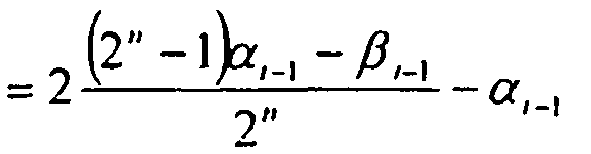$=2\frac{(2^n-1){\alpha }_{i-1}-{\beta }_{i-1}}{2^n}-{\alpha }_{i-1}$
  β t	$=2\frac{(2^n-1){\alpha }_{i-1}-{\beta }_{i-1}}{2^n}+{\beta }_{i-1}$

• So β increases while α decreases. Consider for example the vector superposition in Fig. 11.a. By applying the operator ⁴ H the vector superposition becomes the superposition of Fig. 11.b. Applying the entanglement operator U _F with x=001, the vector superposition of Fig. 11.c is produced and, after the application of D _n ⊗I, the superposition is the one depicted in Fig. 11.d. Here, the probability amplitudes of non-interesting vectors are not null, but they are very small.
• Suppose to apply operator U _F again: the resulting superposition is reported in Fig. 11.e. Then, by applying D _n ⊕I, we obtain the vector linear combination of Fig. 11.f.
• We can observe that the probability amplitude of the desired vectors has increased in modulus. This means a greater probability to measure vectors |0010> or |0011>.
• If we do measurement after h repetitions of operator D _n .U _F , what is the probability P(h) to measure vectors |x>⊗|0> or |x>⊗|1>? We can show that the: $$P^{\prime }\left(h\right)=O\left(2^{-n/2}\right)$$

  
• The quantum block is repeated only 1 time with a sufficiently large h=O(2 ^n/2). So, the final collected basis vector is unique.
Information Analysis A3. Introductory example: Information Analysis of Grover's algorithm
• Let us consider the operator that encoding the input function as: $$U_F=\left[\begin{array}{cccccccc}I& 0& 0& 0& 0& 0& 0& 0\\ 0& \mathrm{<figure-callout\; id="0"\; label="C"\; filenames="imgf0007.png,imgf0010.png"\; state="\{\{state\}\}">C</figure-callout>}& 0& 0& 0& 0& 0& 0\\ 0& 0& I& 0& 0& 0& 0& 0\\ 0& 0& 0& I& 0& 0& 0& 0\\ 0& 0& 0& 0& I& 0& 0& 0\\ 0& 0& 0& 0& 0& I& 0& 0\\ 0& 0& 0& 0& 0& 0& I& 0\\ 0& 0& 0& 0& 0& 0& 0& I\end{array}\right]$$

  
• Table 1 represents a general iteration algorithm for information analysis of Grover's QA. In Tables 2 and 3 two iterations of this algorithm are reported. From these tables we observe that:
1. 1. The entanglement operator in each iteration increases correlation among the different qubits;
2. 2. The interference operator reduces the classical entropy but, as side effect, it destroys part of the quantum correlation measure by the Von Neumann entropy.
• Grover algorithm builds in several iterations intelligent states (see Eq.(7)). Every iteration firstly encodes the searched function by entanglement, but then partly destroys the encoded information by the interference operator; several iterations are needed in order to conceal both the need to have encoded information and the need to access it. Grover's algorithm is from Searching Group of Algorithms. The Principle of Minimum Classical (Quantum) Entropy in output of QA means success result on intelligent output states. The searching QA's needed checking minimum of Classical Entropy and co-ordination the gap with Quantum Entropy Amount. The ability of co-ordination of these both values characterizes the intelligence of searching QA's.
Decoder
• As in Deutsch's algorithm, when the output vector from the quantum gate has been measured, we must interpret it in order to find x .
• From the analyses we did above, this step is very simple. In fact, it is sufficient to choose a large h in order to get the searched vector | x >⊗|0> or | x >⊗|1> with probability near to 1 . After getting it we encode back into their binary values the first n basis vector in the resulting tensor product, obtaining string x as final answer.
• Therefore, it is evinced that Grover's algorithm can be used in search problems.
• A search problem can always be so stated: given a truth function ƒ: {0.1}" → {0,1} such that there is only one input x ∈ {0,1}" : ƒ(x)= 1 find x : this is exactly the kind of problem that can be solved by the Grover's algorithm.
• Comparing between them the algorithm above analyzed, it is clear that quantum algorithms have the same structure: a collection of vectors is sequentially submitted to a superposition operator, to an entanglement operator and to an interference operator. The resulting set of vectors is analyzed by a measurement block which extract the desired information.
• Finally it must be observed that the differences among quantum algorithms consist essentially in the choice of the interference operator Int, the entanglement operator U _F and of the superposition operator S.
• The input vector is a sort of message that traverses a quantum channel made of three main sub-channels: superposition, entanglement and interference. The entanglement channel is the true input of the algorithm gate. It belongs to a given family depending on the problem to solve and on its input. The superposition and especially the interference channels are chosen in such a way that several measurements effectuated at the end of the channel reveal what kind of entanglement has taken place at the middle of the channel.
• In conclusion, it can be stated that Quantum Algorithms are global random searching algorithms based on the quantum mechanics principles, laws, and quantum effects. In the quantum search, each design variable is represented by a finite linear superposition of classical initial stales, with a sequence of elementary unitary steps manipulate the initial quantum state |i〉 (for the input) such that a measurement of the final state of the system yields the correct output. It begins with elementary classical preprocessing, and then it applies the following quantum experiment: starting in an initial superposition of all possible states, it computes a classical function, applies a Quantum Fast Fourier Transform (QFFT), and finally performs a measurement. Depending on the outcome it may carry out one more similar quantum experiments, or complete the computation with some classical post-processing. Usually, three principle operators, i.e. linear superposition (coherent states), entanglement, and interference, are used in the quantum search algorithm.
• In general form the structure of quantum search algorithm can be described as $$\mathrm{G}={\left[\stackrel{\mathit{Interference}}{\overbrace{\left(Int\otimes I_m\right)}}\circ \underset{\mathrm{Entanglement}}{\underbrace{U_F}}\right]}^{h+1}\circ \left(\underset{\mathrm{Superposition}}{\underbrace{H_n\otimes S_m}}\right)$$

  
• In this quantum algorithms and genetic algorithms structures have the following interrelations: $$\begin{array}{ccc}\mathrm{G}\mathrm{A}:\mathrm{E}\left[m\left(H,t+1\right)\right]\ge \mathrm{m}\left(H,t\right)\hfill & \cdot \underset{\Updownarrow }{\underbrace{\underset{\mathrm{Selection}}{\underbrace{\frac{f\left(H,t\right)}{\bar{f}\left(t\right)}}}\cdot \underset{\mathrm{Crossover}}{\underbrace{\left[1-\stackrel{P_d\left(H,t\right)}{\overbrace{p_c\frac{L\left(H\right)}{N-1}\left(1-\frac{m\left(H,t\right)f\left(H,t\right)}{M\bar{f}\left(t\right)}\right)}}\right]}}}}& \underset{\Updownarrow }{\underbrace{\underset{\mathrm{Mutation}}{\underbrace{{\left(1-p_m\right)}^{\mathrm{O}\left(H\right)}}}}}\hfill \\ \mathrm{Q}\mathrm{A}\left(\mathrm{Gate}\right):\hfill & [\stackrel{\mathrm{Interference}}{\overbrace{\left(Int\otimes I_m\right)}}& {\circ \stackrel{\mathrm{Entanglement}}{\overbrace{U_F}}]}^{h+1}°\left(\underset{\mathit{Superposition}}{\underbrace{H_n\otimes S_m}}\right)\hfill \end{array}$$

  
• In Fig. 12 the structures of GA and QSA are compared. In GA a starting population is randomly generated. Mutation and crossover operators are then applied in order to change the genome of some individuals and create some new genomes. Some individuals are then cut off according to a fitness function and selection of good individuals is done generating a new population. The procedure is then repeated on this new population till an optimum is found.
• By analogy in QSA an initial basis vector is transformed into a linear superposition of basis vector by the superposition operator. Quantum operators such as entanglement and interference then act on this superposition of states generating a new one where some states (the non-interesting) have reduced their probability amplitude in modulus and some other (the most interesting) have increased it. The process is repeated several times in order to get to a final probability distribution where an optimum can be easily observed.
• The quantum entanglement operator acts in analogy to the genetic mutation operator: in fact it maps every basis vector in the entering superposition into another basis vector by flipping some bits in the ket label. The quantum interference operator acts like the genetic crossover operator by building a new superposition of basis states from the interaction of the probability amplitudes of the states in the entering superposition. But the interference operator includes also the selection operator. In fact, interference increases the probability amplitude modulus of some basis states and decreases the probability amplitude modulus of some other ones according to a general principle, that is maximizing the quantity $${\mathrm{\Im }}_T\left(|\mathit{output}\rangle \right)=1-\frac{E_T^{Sh}\left(|\mathit{output}\rangle \right)-E_T^{VN}\left(|\mathit{output}\rangle \right)}{\left|T\right|}$$

  

  with T = {1,...,n}. This quantity is called the intelligence of the output state and measure how the information encoded into quantum correlation by entanglement is accessible by measurement. The role of the interference operator is in fact to preserve the Von Neumann entropy of the entering entangled state and to reduce at its minimum the Shannon entropy, which has been increased to its maximum by the superposition operator. Note that there is a strong difference between GA and QSA: in GA the fitness functions changes with different instances of the same problem, whereas mutation and crossover are always random. In QSA the fitness function is always the same (the intelligence of the output state), whereas the entanglement operator strongly depends on the input function ƒ.
• We propose in this patent to merge the two schemes of GA and QSA undergoing the analogy between them and integrating their peculiarities. The new scheme concerns quantum genetic search algorithms (QGSA) and is depicted in Fig. 13.
• An initial superposition with t random non-null probability amplitude values is firstly generated $$|\mathit{input}\rangle ={\displaystyle \sum _{i=1}^t{c}_i|x_i\rangle }$$

  
• Every ket corresponds to an individual of the population and in the general case is labeled by a real number. So, every individual corresponds to a real number x _i and is implicitly weighted by a probability amplitude value c _i . The action of the entanglement and interference operators is genetically simulated: k different paths are randomly chosen, where each path corresponds to the application of an entanglement and interference operator.
• The entanglement operator consists into an injective map transforming each basis vector into another basis vector. This is done defining a mutation ray ε > 0 and extracting t different values ε₁ ,...,ε _t such that - ε ≤ ε _i ≤ ε. Then the entanglement operator U ^j _F for path j is defined by the following transformation rule: $$|x_i\rangle \stackrel{{\mathrm{U}}_F^j}{\to }|x_i+{\epsilon }_i\rangle$$

  
• When ${\mathrm{U}}_F^j$

  

  acts on the initial linear superposition, all basis vectors in it undergo mutation $$|{\psi }^j\rangle ={\displaystyle \sum _{i=1}^t{c}_{i,j}|x_i+{\epsilon }_{i,j}\rangle }$$

  
• The mutation operator ε can be described as following relation $$\epsilon =\{\begin{array}{lll}1\hfill & \mathit{for}\mathit{}\mathit{bit}\mathit{}\mathit{<figure-callout\; id="0"\; label="permutation"\; filenames="imgf0007.png,imgf0010.png"\; state="\{\{state\}\}">permutation</figure-callout>}\hfill & 0\hfill \\ 0\hfill & \mathit{for}\mathit{}\mathit{bit}\mathit{}\mathit{<figure-callout\; id="1"\; label="permutation"\; filenames="imgf0003.png,imgf0004.png"\; state="\{\{state\}\}">permutation</figure-callout>}\hfill & 1\hfill \\ -1\hfill & \mathit{for}\mathit{}\mathit{phase}\mathit{}\mathit{permutation}\hfill & \hfill \end{array}$$

  
• Suppose there are eight states in the system, encoded in binary as 000, 001. 010, 011, 100, 110, 111. One of possible states that may be in during a computation is $\frac{\mathrm{<figure-callout\; id="2"\; label="i"\; filenames="imgf0006.png,imgf0011.png"\; state="\{\{state\}\}">i</figure-callout>}}{\sqrt{2}}|000\rangle +\frac{1}{\sqrt{2}}|100\rangle +\frac{1}{\sqrt{2}}|110\rangle$

  

  . A unitary transform is usually constructed so that it is performed at the bit level.
• For example, the unitary transformation $\begin{array}{cc}\mathrm{\hspace{1em}}& 01\\ \begin{array}{c}\begin{array}{c}0\end{array}\\ 1\end{array}& \left(\begin{array}{cc}0& 1\\ 1& 0\end{array}\right)\end{array}$

  

  will switch the state |0〉 to |1〉 and |1〉 to |0〉 (NOT operator).
• Mutation of a chromosome in GA alters one or more genes. It can also be described by changing the bit at a certain position or positions. Switching the bit can be simply carried out by the unitary NOT-transform.
• The unitary transformation that acts, as example on the last two bits will transform the state |1001〉 to state |1011〉 and the state |0111〉 to the state |0101〉 and so on can be described as the following matrix $$\begin{array}{c}00\\ 01\\ 10\\ 11\end{array}\left(\begin{array}{cccc}\stackrel{00}{1}& \stackrel{01}{0}& \stackrel{10}{0}& \stackrel{11}{0}\\ 0& 0& 0& 1\\ 0& 0& 1& 0\\ 0& 1& 0& 0\end{array}\right)$$

  

  is a mutation operator for the set of vectors 0000〉,|0001〉,...,|1111〉.
• A phase shift operator Z can be described as the following $Z:\begin{array}{l}|0\rangle \to |0\rangle \\ |\begin{array}{c}1\rangle \end{array}\to -|1\rangle \end{array}$

  

  and operator $Y:\begin{array}{l}|0\rangle \to |1\rangle \\ |\begin{array}{c}1\rangle \end{array}\to -|0\rangle \end{array}$

  

  is a combination of negation NOT and a phase shift operator Z.
• Remark 1. As example, the following matrix $$\begin{array}{c}00\\ 01\\ 10\\ 11\end{array}\left(\begin{array}{cccc}\stackrel{00}{1}& \stackrel{01}{0}& \stackrel{10}{0}& \stackrel{11}{0}\\ 0& 1& 0& 0\\ 0& 0& 0& 1\\ 0& 0& 1& 0\end{array}\right)$$

  

  operates a crossover on the last two bits transforming 1011 and 0110 in 1010 and 0111, where the cutting point is at the middle (one-point crossover).
• The two-bit conditional phase shift gate has the following matrix form $$\begin{array}{c}00\\ 01\\ 10\\ 11\end{array}\left(\begin{array}{cccc}\stackrel{00}{1}& \stackrel{01}{0}& \stackrel{10}{0}& \stackrel{11}{0}\\ 0& 1& 0& 0\\ 0& 0& 1& 0\\ 0& 0& 0& e^{i\phi }\end{array}\right)$$

  

  and the controlled NOT (CNOT) gate that can created entangled states is described by the following matrix: $$\begin{array}{r}\mathit{CNOT}:|00\rangle \to |00\rangle \\ |01\rangle \to |01\rangle \\ |10\rangle \to |11\rangle \\ |11\rangle \to |10\rangle \end{array}\Rightarrow \begin{array}{c}00\\ 01\\ 10\\ 11\end{array}\left(\begin{array}{cccc}\stackrel{00}{1}& \stackrel{01}{0}& \stackrel{10}{0}& \stackrel{11}{0}\\ 0& 1& 0& 0\\ 0& 0& 0& 1\\ 0& 0& 1& 0\end{array}\right)$$

  
• The interference operator Int ¹ is chosen as a random unitary squared matrix of order t whereas the interference operators for the other paths are generated from Int ¹ according to a suitable law. Examples of such matrices are the Hadamard transformation matrix H _t and the diffusion matrix D _t , that have been defined above, but many other ones can be built. The application of entanglement and interference operators produces a new superposition of maximum length t: $$|{\mathit{output}}^j\rangle ={\displaystyle \sum _{i=1}^t{c^{\prime }}_{i,j}|x_i+{\epsilon }_{i,j}\rangle }$$

  
• The average entropy value for this state is now evaluated. Let E(x) be the entropy value for individual x. Then $$E\left(|{\mathit{output}}^j\rangle \right)={\displaystyle \sum _{i=1}^t{\Vert {c^{\prime }}_{i,j}\Vert }^{2}E\left(x_i+{\epsilon }_{i,j}\right)}$$

  
• The average entropy value is calculated by averaging every entropy value in the superposition with respect to the squared modulus of the probability amplitudes.
• According to this sequence of operations, k different superpositions are generated from the initial one using different entanglement and interference operators. Every time the average entropy value is evaluated. Selection consists in holding only the superposition with minimum average entropy value. When this superposition is obtained, it becomes the new input superposition and the process starts again. The interference operator that has generated the minimum entropy superposition is hold and Int ¹ is set to this operator for the new step. The computation stops when the minimum average entropy value falls under a given critical limit. At this point measurement is simulated, that is a basis value is extracted from the final superposition according to the squared modulus of its probability amplitude.
• The whole algorithm is resumed on Fig. 14 in the followings:
1. 1. $|\mathit{input}\rangle ={\displaystyle \sum _{i=1}^t{c}_i|x_i\rangle }$
   
   with x _i random real numbers and c _i random compiex numbers such that ${\displaystyle \sum _{i=1}^t{\Vert c_i\Vert }^2}=1$
   
   ; Int ¹ unitary operator of order t randomly generated;
2. 2. $\bar{A}=\left(\begin{array}{c}{\displaystyle \sum _{i=1}^t{c}_i|x_i+{\epsilon }_{i,1}\rangle }\\ {\displaystyle \sum _{i=1}^t{c}_i|x_i+{\epsilon }_{i,2}\rangle }\\ \cdots \\ {\displaystyle \sum _{i=1}^t{c}_i|x_i+{\epsilon }_{i,k}\rangle }\end{array}\right)$
   
   with -ε≤ε _i,j ≤ε randomly generated and ∀i ₁ ,i ₂ ,j:x _{i 1} +ε _{i 1 ,j} ≠x _{i 2} +ε _{i 2 ,j} ;
3. 3. $\bar{B}=\left(\begin{array}{c}\mathrm{I}\mathrm{n}{\mathrm{<figure-callout\; id="1"\; label="t"\; filenames="imgf0003.png,imgf0004.png"\; state="\{\{state\}\}">t</figure-callout>}}^1{\displaystyle \sum _{i=1}^t{c}_i|x_i+{\epsilon }_{i,1}\rangle }\\ \mathrm{I}\mathrm{n}{\mathrm{<figure-callout\; id="2"\; label="t"\; filenames="imgf0006.png,imgf0011.png"\; state="\{\{state\}\}">t</figure-callout>}}^2{\displaystyle \sum _{i=1}^t{c}_i|x_i+{\epsilon }_{i,2}\rangle }\\ \cdots \\ \mathrm{I}\mathrm{n}{\mathrm{t}}^k{\displaystyle \sum _{i=1}^t{c}_i|x_i+{\epsilon }_{i,k}\rangle }\end{array}\right)=\left(\begin{array}{c}{\displaystyle \sum _{i=1}^t{c^{\prime }}_{i,1}|x_i+{\epsilon }_{i,1}\rangle }\\ {\displaystyle \sum _{i=1}^t{c^{\prime }}_{i,2}|x_i+{\epsilon }_{i,2}\rangle }\\ \cdots \\ {\displaystyle \sum _{i=1}^t{c^{\prime }}_{i,k}|x_i+{\epsilon }_{i,k}\rangle }\end{array}\right)$
   
   with Int ^j unitary squared matrix of order t ;
4. 4. $|{\mathit{output}}^{\ast }\rangle ={\displaystyle \sum _{i=1}^t{c^{\prime }}_{i,j^{\ast }}|x_i+{\epsilon }_{i,j^{\ast }}\rangle }$
   
   with $j^{\ast }=\arg \left(\min \left\{{\displaystyle \sum _{i=1}^t{\Vert {c^{\prime }}_{i,j}\Vert }^{2}E\left(x_i+{\epsilon }_{i,j}\right)}\right\}\right)$
   
   ;
5. 5. ${\bar{E}}^{\ast }={\displaystyle \sum _{i=1}^t{\Vert {c^{\prime }}_{i,j^{\ast }}\Vert }^{2}E\left(x_i+{\epsilon }_{i,j^{\ast }}\right)}$
   
6. 6. If E̅* < E ^t and information risk increment is lower than a pre-established quantity Δ then extract x _i* + ε _i*,j* from the distribution $\{\left(x_i+{\epsilon }_{i,j^{\ast }},{\Vert {c^{\prime }}_{i,j^{\ast }}\Vert }^2\right)$
   
   ;
7. 7. Else set |input〉 to | output *〉, Int ⁱ to Int ^j* and go back to step 2.
• Remark 2. Step 6 includes methods of accuracy estimation and reliability measurements of the successful result.
• The simulation of quantum search algorithm is represented through information flow analysis, information risk increments and entropy level estimations:
1. 1) Applying a quantum gate G on the input vector stores information into the system state, minimizing the gap between the classical Shannon entropy and the quantum von Neumann entropy;
2. 2) Repeating said of applying for calculation (estimation) of information risk increments (see below, Remark 3);
3. 3) Measuring said basis vector for estimation the level of average entropy value;
4. 4) Decoding said basis vector of successful result for computation time stopping when the minimum average entropy value falls under a given critical level limit.
• Remark 3. The information risk increments are calculated (estimated) according to the following formula: $$-\sqrt{r\left(W^2\right)2I\left(\tilde{p}:p\right)}\le \left(\delta r=\tilde{r}-r\right)\le \sqrt{\tilde{r}\left(W^2\right)2I\left(p:\tilde{p}\right)}$$

  

  
  where:
• W is the loss function;
• r(W ²)= ∬W ² p(x,θ)dxdθ is an average risk for the corresponding probability density function p(x,θ);
• x = (x₁,...x _n ) is a vector of measured values;
• θ is an unknown parameter;
• $I\left(p:\tilde{p}\right)={\displaystyle \iint p\left(x,\theta \right)\ln \frac{p\left(x,\theta \right)}{\tilde{p}\left(x,\theta \right)}dxd\theta }$
  
  is the relative entropy (the KullbackLeibier measure of information divergence ).
• As stated above, a GA searches for a global optimum in a single solution space. In order to clearly understand the meaning of this statement, further clarifications follows.
• A detailed description of the structures of GA and QSA algorithms is showed in Fig. 15. In the GA search, a solution space 301 leads to an initial position (input) 302. The initial position 302 is coded into binary strings using a binary coding scheme 310. GA operators as selection 303, crossover 304, and mutation 305 are applied to the coded strings to generate a population. Through a fitness function 306 (such as a fitness function based on minimum entropy production rate or some other desirable property) a global optimum for the single space 301 is found.
• Example. The "single solution space" includes any possible coefficient gains of PID controller of plant under stochastic disturbance with fixed statistical properties as the correlation function and probability density function. After stochastic simulation of dynamic behaviour of plant under stochastic excitation with GA we can received the optimal coefficient gains of intelligent PID controller only for stochastic excitation with fixed statistical characteristics. In this case we define the "single space of possible solutions" as 301. If we use stochastic excitation on plant with another statistical characteristics then intelligent PID controller do not can realize control law with fixed KB. In this case we define a new space of possible solutions as 350.
• Remark 4. If we want the universal look-up table for intelligent PID controller from many single solution spaces, then the application of GA do not give us a final corrected result (GA - operators not include superposition and quantum correlation as entanglement). GA give the global optimum on the single solution space. In this case we loss the important information about statistical correlation between coefficient gains in the universal look-up table.
• By contrast, in the QSA shown in Fig. 15, a group of N solution spaces 350 arc used to create an initial position (input) 351. Quantum operators such as superposition 352, entanglement 353, and interference 354 operate on the initial position to produce a measurement. Superposition is created using a Hadamard transformation 361 (one-bit operation). Entanglement is created through a Controlled-NOT (CNOT) operation 362 (a two-bit operation). Interference is created through a Quantum Fourier Transform (QFT) 363. Using the quantum operators, a universal optimum for covering all the spaces in the group 350 is found.
• Remark 5. Thus, the classical process of selection is loosely analogous to the quantum process of creating a superposition. The classical process of crossover is loosely analogous to the quantum process of entanglement. The classical process of mutation is loosely analogous to the quantum process of interference.
• Fig. 16 shows a general structure of a QSA having a conceptual level 400, a structure level 401, a hardware level 402, and software level 403.
• At the conceptual level 400, an initial state 410 is provided to a process block 420 that creates a superposition of states. The superposition of states is provided to a process block 430 that provides a unitary operator U _ƒ to the entanglement. An output of the process block 430 is provided to a solution block 440 that computes an interference of solutions. An output of the solution block 440 is provided to observation/measurement block 460.
• At the structure level, an input is coded as a series of quantum bits (qubits) are prepared in an initial state (e.g., a logical zero state) and provided that are provided to a Hadamard Transform Matrix 421 to produce the superposition. The superposition from the matrix 421 to provide to the operator U _f that produce the entanglement where U _f is in general case a solution to the Schrödinger equation in a process block 431. An output from the process block 431 is provided to a Quantum Fourier Transform (QFT) to provide the interference. The output of the QFT 441 is provided to a Transform Matrix 451. An output of the Transform Matrix 451 is provided as a solution of quantum searching process with maximum probability amplitude 461.
• At the hardware level, the superposition 420 is produced by rotation gates 422, the operator U _f is implemented as a consequence of elementary gate operations and CNOT-gates 432, the QFFT 441 is implemented as a consequence of Hadamard and Permutation (P) operator gates, and the Transform Matrix 451 is implemented using rotation gates 452.
• Fig. 17 illustrates the QSA as an architecture involving the sequence from an initial state, through the creation of superposition. Entanglement is applied to the superposition using quantum parallelism inherent a coherent quantum system with entangled states. The parallelism collapsed when interference is introduced to produce a superposition of solutions through the QFFT. Fig. 17 illustrates these processes by comparing the classical double slit experiment to logical quantum operations and to the quantum search operations.
• Remark 6. In the classical double slit, a source creates a particle having an initial superposition of states. This is analogous to the quantum algorithm operation of applying a Hadamard (rotation gates) transform to a qubit initial to an eigenstate. Returning to the double slit, entanglement is produced with the particle passes through the slits. This corresponds to the process of operating on the superposition using the unitary operator U _f . Again returning to the double slit, interference is produced when the entangled particles strike a photographic film placed behind the slits to produce an interference pattern (a superposition of solutions). This corresponds to the QFFT. Finally, selection of the desired solution corresponds to choosing the largest probability from the QFFT (that is, the brightest line produced on the film).
• The use of the QSA in connection with a GA or FNN is shown Fig. 18. A generator of initial states 604 works in connection with the GA 605 and, optionally a fuzzy neural network (FNN) 603, to produce a set of initial states. The initial states are provided to a Hadamard transform 602 to produce a superposition of states 601. The superposition of classical states is provided to a process block 606 that introduce entanglement through the use of operators such as a CNOT. An output from the process block 606 is provided to an interference block 607 that computes an interference of the entanglement states using QFFT. An output from the interference block 607 is provided block to a measurement/observation block 608 which selects a desired solution from the superposition of solutions computed by the block 607.
• An output from the measurement/observation block 608 is provided to a decision-making block 609. The decision block 609 makes decisions such as inputs for the generator of initial states 604 and, optionally, a new fitness function for the GA 605. The decision block 609 can also provide data to, and receive data from a decoding block 610. The decoding block 610 can communicate with sensors, other control systems, users, etc.
• The basis of quantum computation is obtained from the laws of quantum theory wherein information is something that encoded in the state of a physical system, and a computation is something that can be carried out on an actual physical realizable device.
• A concrete example showing how a random excitation on control object can "kick" the single space of solutions for fuzzy controller is described in the followings.
• Example. The KB of the intelligent suspension control system was received with GA and with stochastic simulation using the random Gaussian signal as road. After on-line simulation with fuzzy controller we use another two real road signal (road measurements in Japan). The results of simulation for pitch angles in Fig. 20 and 21 are shown. Fig. 20 shows that the changing in statistical characteristics of roads (see Fig. 19) kick the single space of solutions for fuzzy controller.
• In this case we must repeat the simulation with GA and use another single space of solution with the fitness function as entropy production for fuzzy controller with non-Gaussian excitation on control object.
• More in details, we are applying GA to minimization of the dynamic behavior of the dynamic system (Plant), and to minimization of entropy production rate. We are using different kinds of random signals (as a stochastic disturbances) which are represents the profiles of roads. Some of this signals were measured from real roads, in Japan, and some of them were created using stochastic simulations with forming filters based on FPK (Fokker - Planck - Kolmogorov) equation. On Fig. 19 three typical road signals are presented. Charts 1901, 1902, 1903 represents changing rates of the signals. Assigned time scale is calculated the way that simulates the vehicle speed of 50kph. First two signals (HouseWC) and (HouseEC) are the measured real roads of Japan. Third signal is a Gaussian road obtained by stochastic simulation with the fixed type of the correlation function. We can see that the dynamic characteristics of this roads are similar (see charts (A)), but statistical characteristics of HouseWC road are very different from statistical characteristics of Gaussian and of HouseEC roads (see charts (B)). HouseWC road represents so called Non-Gaussian (color) stochastic process.
• Big difference in the statistical characteristics of the road signals gives us completely different responses from dynamic system and as a result, required different control solutions.
• Figs. 20 and 21 illustrate the dynamic and thermodynamic response of the suspension system (P_LANT) to the mentioned above excitations. Charts (a) represent dynamic behaviour of the pitch angle of the vehicle under HouseWC (linel), HouseEC (line 2) and Gaussian (line 3) roads. The knowledge base as a look-up table for fuzzy controller in this case was obtained using Gaussian road signal, and then applied to the House WC and HouseEC roads. We see that system response from the roads with the same characteristics are similar, which means that GA has found the optimum solution for Gaussian-like signal shapes, but response obtained from the system with HouseWC road is a completely different signal. For this Non-Gaussian road we need new control GA strategy that differs from the mentioned above e.g. it requires solution from different single space of solutions. On the phase portrait (Charts (b)) the difference of system responses is more visible.
• It is desirable, however, to search for a global optimum in multiple solution spaces to find a "universal" optimum. A quantum genetic search algorithm provides the ability to search multiple spaces simultaneously (as described below).
• Fig. 2 shows a modified version of the intelligent control system of the invention, wherein a Quantum Genetic Search Algorithm (QGSA) is interposed between the GA and the FNN. The QGSA searches several solution spaces, simultaneously, in order to find a universal optimum, that is, a solution that is optimal considering all solution spaces.
Method for controlling a process and relative controller
• The QGSA can be used in a method for controlling a process (PLANT) driven by a control signal (U*). The control signal (U*) is calculated as a function of a parameter adjustment signal (CGS) and an error signal (ε), obtained as the difference between the state of the process (X) and of a reference signal (Y).
• The object of the method is to minimize a certain physical quantity, which can be for example the entropy production of the controlled process. To reach this goal, a signal (S) representative of the quantity to be minimized is derived by processing paired values of said state (X) of the process and said control signal (U*).
• The method of the invention advantageously uses the Quantum Genetic Search Algorithm to find the best control signal (U*) to input the process to control. Such a control signal is produced by a controller with an adjustable transfer characteristic as a function of a vector of values to assign to the parameters of the controller.
• So the problem of controlling a process can be restated in the following manner: find a vector of values that minimizes a certain quantity which is function of said vector, i.e. find a vector that minimizes a certain vector function.
• Therefore, it is evident that Genetic Algorithms are of great importance in methods for controlling a process and how a Quantum Genetic Search Algorithm can be effectively used in such applications.
• First a correction signal (K2) is periodically calculated from a set of several different values of said control signal (U*), that minimize said derived signal (S) to be minimized.
• This correction signal (K2) is calculated applying to a set of vectors representing as many different control signals (U*) a Quantum Genetic Search Algorithm, using a fitness function that is as greater as lower the quantity to be minimized is.
• Finally such correction signal (K2) is fed to a fuzzy neural network that produces said parameter adjustment signal (CGS) provided together the error signal (ε) to a fuzzy processor, which adjusts the transfer characteristic of the controller.
• Many different embodiments of this method can be implemented by changing the physical quantity to be minimized, which can be for example the difference between the Shannon and von Neumann Entropy or the Heisenberg uncertainty or, more specifically, for an internal combustion engine, the entropy production of the thermodynamic process.
• It is also possible to have a suitably adapted Quantum Genetic Search Algorithm of the invention choosing the interference and entanglement operators according to any of quantum problems: for example it is possible to choose such operators according to Grover's problem or a Shor's problem.
• A preferred embodiment of the method of the invention consists in running a Genetic Algorithm with the set of vectors representing as many different control signals (U*), producing a temporarily correction signal (K), which is elaborated by a Quantum Genetic Search Algorithm. This embodiment is preferred because in that way the convergence of the Quantum Genetic Search Algorithm is faster.
• A structure of a preferred hardware embodiment of the method of the invention is depicted in Fig. 2. The process (PLANT) driven by a control signal u* is placed in a classical feed-back control loop together with a PID controller. The PID produce the driving signal u* depending on an error signal ε calculated as a function of a state of the process X and of a reference signal Y.
• A circuit block derives a signal s representative of a quantity to be minimized, which can be the entropy production for example, calculated by processing paired values of the state X of the process and the control signal U*.
• The signal S can be input into a circuit QGSA implementing a Quantum Genetic Search Algorithm, outputting a correction signal K2, or can be first managed by a circuit GA implementing a Genetic Algorithm, that produces a temporary correction signal K to input the QGSA circuit.
• Although the circuit implementing the GA is not essential in the structure depicted in Fig. 2, because a Quantum Genetic Search Algorithm of the invention may be considered as a "generalization" of a Genetic Algorithm, generally the circuit GA implementing a Genetic Algorithm is present in the system's architecture.
• This because the GA circuit produces structured data for the Quantum Genetic Search Algorithm, allowing a faster convergence of the algorithm. Generally it can be stated that a Genetic Algorithm produces optimal solution from single space of solution: it means that with the GA circuit implementing a Genetic Algorithm we can compress information from single space of solution with the guarantee of the safety of informative parameters in signal K. The quantum search on structured data guarantees the search of successful solution with higher probability and accuracy than on unstructured data.
• A fuzzy neural network FNN produces a driving signal depending on values of the correction signal K2 output by the QGSA, and a fuzzy controller FC adjusts the transfer characteristic of the classical PID controller depending on values of the driving signal and of the error signal ε.

Claims (12)

1. A method of controlling a process (P_LANT) driven by a control signal (U*) for producing a corresponding output, comprising
   producing an error signal (ε) as a function of a state of said process (X) and of a reference signal (Y),
   generating a control signal (U*) as a function of said error signal (ε) and of a parameter adjustment signal (CGS) and feeding it to said process (P_LANT),
   deriving a signal (S) representative of a quantity to be minimized calculated by processing paired values of said state (X) of the process and said control signal (U*),
   calculating a correction signal (K2) from a set of several different values of said control signal (U*), that minimize said derived signal (S) to be minimized,characterized in that it comprises the steps of
   calculating said parameter adjustment signal (CGS) by means of a fuzzy controller based on said error signal (ε) and on a driving signal produced by a fuzzy neural network depending on values of said correction signal (K2),
   said correction signal (K2) is periodically calculated by a Quantum Genetic Search Algorithm consisting in a merging of a genetic algorithm and a quantum search algorithm comprising the following steps:

   producing an initial set of vectors representing in vector form several different possible values of said correction signal (K2);

   calculating a second set of vectors by a linear superposition of vectors of said initial set;

   performing on vectors of said second set a certain number of parallel computations of random entanglement operations and random interference operations according to a quantum search algorithm, producing as many vectors representatives of values of said control signal (U*) of the process (P_LANT);

   associating to each resulting value of said parallel computations a fitness function as greater as lower the quantity to be minimized (S), calculated using paired values of said control signal (U*) and state (X) of the process (P_LANT) corresponding to the considered resulting value, is;

   performing a selection operation of resulting values of said parallel computations according to a genetic algorithm using said fitness functions;

   calculating said correction signal (K2) as the final result of said selection.
2. The method according to claim 1 wherein said initial set of vectors is obtained by
   producing a first set of vectors representing several different possible values of said correction signal (K2);
   applying a genetic algorithm (GA) on said first set of vectors calculating a temporary correction signal (K) using a fitness function as greater as lower the quantity to be minimized (S), calculated using paired values of said control signal (U*) and state (X) of the process (P_LANT) corresponding to the considered resulting value, is;
   producing said initial set as a collection of the different values of said temporary correction signal (K).
3. The method of claims 1 or 2 wherein said derived signal (S) to be minimized represents the information distance between Shannon entropy and von Neumann entropy of pairs of said control signal (U*) and state (X);
   said fitness function is the information intelligence measure of each resulting value of said parallel computations.
4. The method of claims 1 or 2 wherein said derived signal (S) to be minimized is the Heisenberg uncertainty.
5. The method according to one of the preceding claims wherein said quantum search algorithm is a Grover quantum search algorithm.
6. The method according to one of the preceding claims wherein said linear superposition is a Hadamard rotation.
7. The method according to one of the preceding claims wherein said interference operation is obtained by an interference operator constituted with a random unitary squared matrix implementing a Fast Quantum Fourier Transform.
8. A controller of a process (P_LANT) driven by a control signal (U*) comprising
   a first circuit block producing an error signal (ε) as a function of a state of said process (X) and of a reference signal (Y),
   a second circuit block with adjustable transfer characteristic generating a control signal (U*) as a function of said error signal (ε) and feeding it to said process (P_LANT),
   characterized in that said it comprises
   a third circuit block deriving a signal (S) representative of a quantity to be minimized calculated by processing paired values of said state (X) of the process and said control signal (U*),
   a fourth circuit block calculating a correction signal (K2) from a set of several different values of said control signal (U*), that minimize said derived signal (S) representing the entropy production capacity,
   a fuzzy neural network producing a driving signal depending on values of said correction signal (K2),
   a fuzzy controller adjusting the transfer characteristic of said second circuit block depending on values of said driving signal and said error signal (ε),
   said fourth circuit block periodically calculates said correction signal (K2) by a Quantum Genetic Search Algorithm consisting in a merging of a genetic algorithm and a quantum search algorithm by performing the following operations:

   producing an initial set of vectors representing in vector form several different possible values of said correction signal (K2);

   calculating a second set of vectors by a linear superposition of vectors of said initial set;

   performing on vectors of said second set a certain number of parallel computations of random entanglement operations and random interference operations according to a quantum search algorithm, producing as many vectors representatives of values of said control signal (U*) of the process (P_LANT);

   associating to each resulting value of said parallel computations a fitness function as greater as lower the quantity to be minimized (S), calculated using paired values of said control signal (U*) and state (X) of the process (P_LANT) corresponding to the considered resulting value, is;

   performing a selection operation of resulting values of said parallel computations according to a genetic algorithm using said fitness functions;

   calculating said correction signal (K2) as the final result of said selection.
9. The controller of the preceding claim wherein said initial set of vectors is obtained by
   producing a first set of vectors representing several different possible values of said correction signal (K2);
   calculating a temporary correction signal (K) by a genetic algorithm (GA) applied on said first set of vectors using a fitness function as greater as lower the quantity to be minimized (S), calculated using paired values of said control signal (U*) and state (X) of the process (P_LANT) corresponding to the considered resulting value, is;
   producing said initial set as a collection of the different values of said temporary correction signal (K).
10. The controller according to one of claims 8 or 9 wherein said process to control (P_LANT) is an internal combustion engine and said third circuit derives a signal (S) representative of the entropy production of said engine.
11. The controller according to one of claims 8 or 9 wherein said derived signal (S) to be minimized represents the information distance between Shannon entropy and von Neumann entropy of pairs of said control signal (U*) and state (X);
    said fitness function is the information intelligence measure of each resulting value of said parallel computations.
12. The controller according to one of claims from 8 to 11 wherein said second circuit block is a proportional-integral-differential controller (PID).

Images