EP1171028B1 - System for determining haemodynamic indices by use of tomographic data - Google Patents
System for determining haemodynamic indices by use of tomographic data Download PDFInfo
- Publication number
- EP1171028B1 EP1171028B1 EP00912409A EP00912409A EP1171028B1 EP 1171028 B1 EP1171028 B1 EP 1171028B1 EP 00912409 A EP00912409 A EP 00912409A EP 00912409 A EP00912409 A EP 00912409A EP 1171028 B1 EP1171028 B1 EP 1171028B1
- Authority
- EP
- European Patent Office
- Prior art keywords
- tissue
- flow
- organ
- tracer
- determined
- Prior art date
- Legal status (The legal status is an assumption and is not a legal conclusion. Google has not performed a legal analysis and makes no representation as to the accuracy of the status listed.)
- Expired - Lifetime
Links
Images
















Classifications
-
- G—PHYSICS
- G06—COMPUTING OR CALCULATING; COUNTING
- G06T—IMAGE DATA PROCESSING OR GENERATION, IN GENERAL
- G06T7/00—Image analysis
- G06T7/0002—Inspection of images, e.g. flaw detection
- G06T7/0012—Biomedical image inspection
-
- A—HUMAN NECESSITIES
- A61—MEDICAL OR VETERINARY SCIENCE; HYGIENE
- A61B—DIAGNOSIS; SURGERY; IDENTIFICATION
- A61B5/00—Measuring for diagnostic purposes; Identification of persons
- A61B5/05—Detecting, measuring or recording for diagnosis by means of electric currents or magnetic fields; Measuring using microwaves or radio waves
- A61B5/055—Detecting, measuring or recording for diagnosis by means of electric currents or magnetic fields; Measuring using microwaves or radio waves involving electronic [EMR] or nuclear [NMR] magnetic resonance, e.g. magnetic resonance imaging
-
- A—HUMAN NECESSITIES
- A61—MEDICAL OR VETERINARY SCIENCE; HYGIENE
- A61B—DIAGNOSIS; SURGERY; IDENTIFICATION
- A61B6/00—Apparatus or devices for radiation diagnosis; Apparatus or devices for radiation diagnosis combined with radiation therapy equipment
- A61B6/50—Apparatus or devices for radiation diagnosis; Apparatus or devices for radiation diagnosis combined with radiation therapy equipment specially adapted for specific body parts; specially adapted for specific clinical applications
- A61B6/507—Apparatus or devices for radiation diagnosis; Apparatus or devices for radiation diagnosis combined with radiation therapy equipment specially adapted for specific body parts; specially adapted for specific clinical applications for determination of haemodynamic parameters, e.g. perfusion CT
-
- A—HUMAN NECESSITIES
- A61—MEDICAL OR VETERINARY SCIENCE; HYGIENE
- A61B—DIAGNOSIS; SURGERY; IDENTIFICATION
- A61B6/00—Apparatus or devices for radiation diagnosis; Apparatus or devices for radiation diagnosis combined with radiation therapy equipment
- A61B6/50—Apparatus or devices for radiation diagnosis; Apparatus or devices for radiation diagnosis combined with radiation therapy equipment specially adapted for specific body parts; specially adapted for specific clinical applications
- A61B6/508—Apparatus or devices for radiation diagnosis; Apparatus or devices for radiation diagnosis combined with radiation therapy equipment specially adapted for specific body parts; specially adapted for specific clinical applications for non-human patients
-
- G—PHYSICS
- G01—MEASURING; TESTING
- G01R—MEASURING ELECTRIC VARIABLES; MEASURING MAGNETIC VARIABLES
- G01R33/00—Arrangements or instruments for measuring magnetic variables
- G01R33/20—Arrangements or instruments for measuring magnetic variables involving magnetic resonance
- G01R33/44—Arrangements or instruments for measuring magnetic variables involving magnetic resonance using nuclear magnetic resonance [NMR]
- G01R33/48—NMR imaging systems
- G01R33/54—Signal processing systems, e.g. using pulse sequences ; Generation or control of pulse sequences; Operator console
- G01R33/56—Image enhancement or correction, e.g. subtraction or averaging techniques, e.g. improvement of signal-to-noise ratio and resolution
- G01R33/5601—Image enhancement or correction, e.g. subtraction or averaging techniques, e.g. improvement of signal-to-noise ratio and resolution involving use of a contrast agent for contrast manipulation, e.g. a paramagnetic, super-paramagnetic, ferromagnetic or hyperpolarised contrast agent
-
- A—HUMAN NECESSITIES
- A61—MEDICAL OR VETERINARY SCIENCE; HYGIENE
- A61B—DIAGNOSIS; SURGERY; IDENTIFICATION
- A61B6/00—Apparatus or devices for radiation diagnosis; Apparatus or devices for radiation diagnosis combined with radiation therapy equipment
- A61B6/02—Arrangements for diagnosis sequentially in different planes; Stereoscopic radiation diagnosis
- A61B6/03—Computed tomography [CT]
- A61B6/037—Emission tomography
-
- G—PHYSICS
- G01—MEASURING; TESTING
- G01R—MEASURING ELECTRIC VARIABLES; MEASURING MAGNETIC VARIABLES
- G01R33/00—Arrangements or instruments for measuring magnetic variables
- G01R33/20—Arrangements or instruments for measuring magnetic variables involving magnetic resonance
- G01R33/44—Arrangements or instruments for measuring magnetic variables involving magnetic resonance using nuclear magnetic resonance [NMR]
- G01R33/48—NMR imaging systems
- G01R33/54—Signal processing systems, e.g. using pulse sequences ; Generation or control of pulse sequences; Operator console
- G01R33/56—Image enhancement or correction, e.g. subtraction or averaging techniques, e.g. improvement of signal-to-noise ratio and resolution
- G01R33/563—Image enhancement or correction, e.g. subtraction or averaging techniques, e.g. improvement of signal-to-noise ratio and resolution of moving material, e.g. flow contrast angiography
-
- G—PHYSICS
- G06—COMPUTING OR CALCULATING; COUNTING
- G06T—IMAGE DATA PROCESSING OR GENERATION, IN GENERAL
- G06T2207/00—Indexing scheme for image analysis or image enhancement
- G06T2207/30—Subject of image; Context of image processing
- G06T2207/30004—Biomedical image processing
- G06T2207/30016—Brain
Definitions
- the present invention relates to a system for determining haemodynamic indices of an organ or a part of tissue of a mammal, such as a human being, from a time series of tomographic data, especially data obtained by means of Magnetic Resonance Imaging (MRI).
- the method produces maps of distribution of blood transit time as well as other indices being significant of the dynamics of the capillary tissue flow from tomographic images acquired during rapid bolus injection of a contrast agent or tracer that stays mainly intravascular in the organ.
- the haemodynamic indices may by use of the present method be obtained with a spatial resolution equal to the spatial resolution of the tomographic data.
- the method comprises the steps of conversion of tomographic images into data representing concentrations of contrast agent as a function of time, and the method determines the distribution of flow and mean transit time, either in absolute values or relative to the mean value, whereby the methods facilitates the (i) comparison of relative flow or transit time distributions to that of other tissue (in particular cerebral tissue), such as normal tissue, or (ii) quantification of absolute flow distributions in terms of the associated extraction of a substance with known capillary permeability.
- the use of the methods for examination and monitoring of cerebral conditions of humans are of particular interest, but the method may also be applied to other organs, such as the heart, the liver, kidneys, tumors etc., or to other part of tissue or part of organs.
- Flow and microscopic heterogeneity of flow are believed to be a main determinants of how efficient the delivery of nutrients and pharmaceuticals to tissue takes place.
- diseases where delivery of nutrients such as e.g. oxygen is compromised by flow reduction, determination of flow heterogeneity is therefore crucial to assess the severity of the disease.
- diseases include acute cerebral ischemia, a frequent cause of death and the major cause of adult neurological disability in the Western world.
- the measurement of flow heterogeneity has been limited to the study to superficial vessels in the cortex of anaesthetised animals by high-speed intravital microscopy. There are no pre-existing tools that allow determination flow heterogeneity in deeper structures, or on humans as part of non-invasive, routine diagnostic procedures.
- PET Positron Emission Tomography
- ⁇ stergaard et al. disclose determining a time series of tomographic data, determining a time series of concentration data being indicative of the concentration of the tracer from the time series of tomographic data, and determining a residue function by deconvolution of the time series of tomographic data with the time series of concentration data, and determining a distribution of transit times from the negative slope of the residue function.
- the present invention describes and validates a new, non-invasive method that allows assessment of flow heterogeneity on generally available tomographic equipment (Magnetic Resonance (MR), Computed Tomography (CT), PET). Furthermore, the technique allows indirect assessment of metabolic parameters.
- MR Magnetic Resonance
- CT Computed Tomography
- PET PET
- the technique has high predictive power in terms of disease progression in cerebral diseases such as ischemia, thereby providing the means for rapid assessment of the efficacy of novel therapies.
- haemodynamic indices such as distribution of transit times and parameter characterising said distribution, quantitative haemodynamic parameters obtained from said distribution such as parameters characterising the deviation of said distribution from a reference distribution, as well as other indices being significant of the dynamics of the capillary tissue flow.
- a normal organ e.g. the brain
- an organ having a recognised disease or condition such as having a tumour of an identified tumour type.
- the present invention which is defined by the appended set of claims relates to a system for determining haemodynamic indices of an organ or part of tissue of a mammal including
- the residue function may also be understood as a normalised impulse response function characterising the fraction of the tracer present in the vascular tissue at time t after a perfect, infinitely sharp input of a tracer in the feeding vessel.
- a number of known methods may be applied, such as a Fourier transform, Box transform, but preferably the Singular Value Decomposition is used.
- tomographic data is herein understood as data representing the concentration of the tracer, i.e. being a direct measure of the concentration or being directly proportional to the concentration of the tracer.
- concentration data typically have the same physical dimension.
- the distribution of transit times obtained from this method may be used to determine a probability density function (PDF) of a normalised haemodynamic index, where the index is normalised by the value of the integral of this index.
- PDF probability density function
- One of the haemodynamic indices obtained from the PDF may be a quantitative haemodynamic parameter, such as a parameter obtained from comparison of the determined PDF and a previously determined reference PDF, e.g. obtained by use of the Kolmogorov Smirnov test.
- the comparison between the determined PDF and a reference may also include identification of plateau's of the curve of the PDF, distribution of area under the curve, area under the curve at one or the other side of a cut-off value, etc.
- the predetermined reference PDF used for comparison may have been found for a normal organ (e.g. the brain) or tissue or for an organ having a recognised disease or condition, such as having a tumour of an identified tumour type.
- the present invention relates to a system in which the quantitative parameter may be obtained by performing the steps of determining the impulse response function of the organ or of the part of tissue by deconvolution of the time series of tomographic data with the time series of concentration data, determining the relative tissue flow from the impulse response function of the organ or of the part of tissue, normalising said time series of concentration data with the integral of said time series of concentration data with respect to time, determining the normalised relative tissue flow, respectively the normalised blood volume, of the organ or part of tissue by use of the relative tissue flow and the time series of normalised concentration data, and converting said normalised relative tissue flow, respectively normalised blood volume, to an absolute value for the tissue flow, respectively the blood volume, by means of a previously determined conversion factor, the quantitative haemodynamic parameter being of metabolic significance and determined from the PDF and the absolute tissue flow, respectively the absolute blood volume.
- the normalised relative tissue flow obtained from this method may be used to compare tissue flow determined from successive tomographic scanning of the same mammal in order to monitor the development of a condition of an organ or part of tissue and/or to compare tissue flow of different individuals.
- the comparison may be performed because the data have been normalised which means that they are readily comparable.
- the blood volume is obtained by dividing the blood flow by the mean transit time (MTT) or as the area under the tissue concentration curve (or the impulse response function) of the first pass of the bolus tracer passage.
- MTT mean transit time
- tomographic data may be obtained from a variety of methods, of which MRI and Computed Tomography (CT) are preferred. However, for some applications it may be preferred to use other methods, such as Positron Emission Tomography (PET) or Single Photon Emission Computed Tomography (SPECT).
- PET Positron Emission Tomography
- SPECT Single Photon Emission Computed Tomography
- the above method may further comprise a step, wherein the normalised relative tissue flow, respectively the blood volume, is also normalised with the ratio between body weight of the individual mammal and the injected tracer dose.
- the determined relative tissue flow is furthermore made comparable to determined relative tissue flow from tomography time series of the same individual mammal in which the amount of the injected tracer dose have been changed.
- the relative tissue flow determined for one individual mammal may furthermore be compared to relative tissue flows determined for other individuals.
- the conversion factor may be a factor that is generally applicable for the present method to members of a mammalian specie.
- the conversion factor may be a factor that is generally applicable for the present method to an organ or tissue of the mammalian specie.
- a parameter (E) significant for the local extraction of a substance may be determined by a method further comprising the following steps:
- the substance in question may, e.g., be oxygen, glucose or another important cellular metabolic substance or it may, e.g., be a drug or another substance having a therapeutic effect.
- the normalised relative tissue flow is also normalised with the injected tracer dose being the ratio between tracer amount and body weight of the individual mammal.
- the tomography data for the system according to the invention are preferably obtained by means of magnetic resonance imaging, and the method is furthermore preferably applied to cerebral tissue.
- cerebral tissue it has been found to be advantageous to obtain the tomographic data by means of susceptibility contrast magnetic resonance imaging.
- the tissue may be renal tissue, in particular renal parenchyma tissue.
- the tissue may further include tumour tissue, in particular in case the tissue is cerebral tissue.
- the tracer may be a Gd-chelate, such as Gd-DTPA. It may alternatively be an ultra small iron oxide particle (USPIO) intravascular contrast agent. This is particularly preferred since an USPIO intravascular contrast agent is only transferred to the surrounding tissue to a very limited extend. Thus, the contrast agent is mainly maintained in the blood, whereby the contrast of the resulting MR image is greatly enhanced. This is of particular interest in non-cerebral tissue, such as renal tissue.
- Gd-chelate such as Gd-DTPA
- USPIO ultra small iron oxide particle
- the predetermined conversion factor may be a constant factor applicable for the present method for any organ or any part of tissue of the mammalian specie.
- the predetermined conversion factor is a constant factor applicable for all of cerebral tissue of the mammalian specie, which is strongly indicated from empirical evidence.
- the tomographic data discussed above and used in the present method will normally comprise information pertaining to subregions of sections of the organ or part of tissue and the haemodynamic indices are determined for at least a substantial part of said subregions.
- the data of the subregions may be represented graphically as pixel values (as a gray-scale image or colour image of the section), and the quantitative haemodynamic parameter determined from the tomograpic data may also be represented as images subdivided into a plurality of pixels each representing a quantitative haemodynamic parameter pertaining to one of said subregions.
- the present invention relates to a system for processing of time series of tomographic data pertaining to an organ or a part of tissue according to one or more of the above described methods, said system residing on a computer having means for producing an output representative of at least some of the determined haemodynamic indices.
- the equipment for performing the tomographic data for use in the system according to the present invention is general standard equipment available to such an extent that the method can be applied in routine patient management.
- the determination may be performed easily and rapidly for healthy as well severely ill patients such as patients in coma.
- the method may be used for diagnosis and evaluation of possible further progress of disease whereby a suitable treatment schedule may be applied.
- the present method is useful in connection with detection of heterogeneity of transit times, velocities or flows by means of external detection of tracers in general, whether in biological or technical systems.
- the technique is applicable to the diagnosis and study of a number of diseases, as well as in the development and subsequent monitoring of therapies in these diseases. Examples include:
- the present method produces maps of normalised relative or absolute tissue blood flow, blood volume and absolute blood mean transit time from dynamic, tomographic images acquired during rapid bolus injection of a contrast agent or tracer that stays mainly intravascular in the organ.
- 'blood volume is understood tracer or contrast agent distribution volume per tissue volume. If the distribution volume is less than that of total blood (e.g. only plasma), it is understood that conversion to absolute blood volume can be achieved by knowledge of regional distribution volume characteristics, e.g. haematocrit, or other normalisation by an independent techniques (e.g. positron emission tomography) as presented in this description.
- 'blood flow' refers to flow of tracer or contrast agent distribution volume per tissue volume per unit time, with the aforementioned method of conversion to blood flow.
- 'transit time' refers to the time taken for tracer or contrast agent to traverse the image element, the arrival at which is defined from the arterial input measurement.
- the method determines the distribution of flow and mean transit time, either in absolute values or relative to the mean value.
- the methods further allows the (i) comparison of relative flow distributions to that of normal tissue (here brain) or (ii) quantification of absolute flow distributions in terms of the associated extraction of a substance with known capillary permeability.
- the method and associated software handles various modalities, depending on whether tracer injection changes signal intensity from baseline in a linear or logarithmic fashion upon tracer arrival.
- acquired tomographic images during tracer bolus injection are converted into concentrations as a function of time, with measurement time points spaced equally in time.
- the tissue concentration as a function of time, C t (t) is typically obtained by the formula where S(t 0 ) is the signal intensity before contrast injection (formed as the average of signal intensities up to tracer arrival), S(t) is the signal intensity at time t, and TE is the echo time used in the sequence.
- k is a constant characteristic of the tissue and contrast agent.
- concentrations are assessed directly by the change in longitudinal relaxation rate, ⁇ R 1 , as derived from signal intensity changes where is the relaxivity of the applied contrast agent.
- CT Computed Tomography
- the algorithm For identification of arterial vessels in the image, the algorithm provides the choice of first producing an image that guides this process (2.a.), or proceeding directly to calculation of tissue flow (2.b.)
- the concentration time curve of each image element is fitted to a gamma variate function by nonlinear least-squared regression (by means of a fletcher-algorithm) over the time interval until visible tracer re-circulation occurs (the re-circulation is specified by the user, determining
- the corresponding signal intensity time curve is fed to the program below in the form of an ASCII file.
- the algorithm includes a method to allow comparison of relative tissue blood flow and tissue blood volume in serial examinations in the same subject or animal.
- the area of the arterial input function (as determined by gamma variate fitting above) is set equal to the injected dose (in millimoles) normalised per body weight prior to the deconvolution below.
- subsequent blood volume measurements are divided by the aforementioned, dose-corrected arterial input area.
- relative blood volume is determined as the area under the tissue concentration time curve corresponding to the first-pass of the injected tracer or contrast agent (See e.g. Figure 2 in Example 1), normalised to the arterial input area determined in 3.
- the area is determined both by direct, numerical integration, and by gamma variate fitting (See section 2).
- Equation 4 can be reformulated as a matrix equation
- the equation is (after applying Simpsons rule to the matrix elements ( ⁇ stergaard 1996b)) solved for F t ⁇ R(t) in each pixel by Singular Value Decomposition (SVD), with a cut-off in diagonal eigenvalues at 20% of the maximum value in order to suppress experimental noise typical of tomographic images (signal to noise ratio of the order of 10).
- the noise cut-off of 20 % is user specified.
- SNR signal-to-noise ratio
- a Monte Carlo simulation scheme is provided to optimise the cut-off ( ⁇ stergaard 1996b).
- the algorithm allows independent correction for tracer arrival delays prior to deconvolution by shifting the tissue curve in a given pixel by the delay fitted in 2.a., thereby reducing bias in flow rates due to simple delays of the tissue curve relative to the arterial input curve ( ⁇ stergaard 1996a).
- the algorithm calculates the following quantities, and stores them as digital, floating point images:
- CBF cerebral blood flow
- CBV cerebral blood volume
- relative flows refer to a defined fraction of the mean flow, i.e. a dimensionless quantity, independent of any absolute quantification of flow.
- w(f) be a probability density function (PDF), i.e. has area 1, and has mean value 1 (i.e. describes flows relative to total flow), i.e.
- PDF probability density function
- the resulting distribution of relative flows is recalculated by linear interpolation to determine its values at predefined relative flow values previously determined for normal tissue ( Figure 13b in Example 3).
- the values read f w(f) f w(f) 3.8053 1.65E-03 0.6941 1.4594 2.865 0.0226 0.647 1.5915 2.3306 0.0372 0.6205 1.6279 1.7879 0.0627 0.5969 1.5812 1.5881 0.1198 0.5815 1.351 1.4459 0.1751 0.565 1.3393 1.3535 0.2491 0.5448 1.2367 1.2785 0.3303 0.5262 1.1433 1.1912 0.4058 0.5133 1.0688 1.1106 0.4793 0.5007 0.928 1.0474 0.646 0.4822 0.6559 0.9972 0.7218 0.4689 0.6366 0.9438 0.9032 0.4571 0.4282 0.8981 0.986 0.4416 0.3133 0.8214 1.1098 0.4316 0.0244 0.7794 1.3562 0.42 0
- the program returns digitized images of
- the program combines the relative flow heterogeneity w(f) with absolute flow estimates (See Section 5) to calculate distribution of absolute flows in ml/100ml/min. Furthermore, using the microvascular weighting (For example as demonstrated in Example 1 or in ⁇ stergaard 1998c) and table values for the microvascular dimensions of the organ in question (for brain capillaries e.g. 8 ⁇ m diameter and 120 ⁇ m length), blood volume is converted into capillary surface area, S. The local extraction E of a substance with capillary permeability P (as given by literature values), is then given by:
- This quantity is visualised as a separate image, based on the specified value of P.
- S can be inferred from the blood volume by literature values describing microvascular dimensions and fractions for the relevant organ.
- Cerebral blood flow was determined with magnetic resonance imaging (MRI) of contrast agent bolus passage, and compared the results to those obtained by positron emission tomography (PET).
- MRI magnetic resonance imaging
- PET positron emission tomography
- Six pigs were examined by MRI and PET under normo- and hypercapnic conditions. After dose normalisation and introduction of an empirical constant ⁇ Gd, absolute regional CBF was calculated from MRI. The spatial resolution and the signal-to-noise-ratio of CBF measurements by MRI were better than by the H 2 15 O-PET protocol.
- CBV Cerebral Blood Volume
- CBV cerebral blood volume
- C vol (t) of an intravascular contrast agent within a given volume of interest can be expressed as where C a (t) is the arterial input, F is tissue blood flow and R(t) is the vascular residue function, i.e. the fraction of tracer present in the vascular bed of the VOI at time t after injection of a unit impulse of tracer in its supply vessel.
- Vascular volume was determined by numerically integrating the area under the concentration time curve during the contrast bolus
- the integrated area of the arterial input curve was in each measurement normalised to the injected contrast dose (in mM per kg body weight) in order to compare within and among animals.
- the deconvolution was performed over the range of measurements where the arterial input values exceeded the noise level (usually about 15 seconds). Deconvolution followed smoothing of raw image data by a 3 x 3 uniform smoothing kernel to. The maximum of the deconvolved response curve was assumed proportional to CBF.
- CBV was determined by numerically integrating the concentration time curve from bolus arrival to tracer re-circulation.
- 15 O 2 was produced by the 14 N(d,n) 15 O nuclear reaction by the bombardment of nitrogen gas with 8.4 MeV deuterons using a GE PETtrace 200 cyclotron. 15 O 2 was mixed with hydrogen and passed in a stream of nitrogen gas over a palladium catalyst at 150°C to produce 15 O-water vapour, which was trapped in 10 ml sterile saline. 15 O-CO was prepared by passing 15 O 2 in a stream of nitrogen gas over activated carbon at 900 °C. The 15 O-CO was piped directly to a 500 ml vial in a dose calibrator situated close to the PET scanner. Upon decay to the required radioactivity, the 15 O-CO was administered to the pig as described below.
- 15 O-Butanol was prepared by the reduction of 15 O 2 with tri-n-butyl borane immobilised on an aluminum solid phase matrix. The product was purified by transfer of the resulting radioactivity with 10 ml H 2 O onto a C18 solid phase extraction column. The 15 0-butanol was subsequently eluted into a sterile vial with 10 ml 20% ethanol.
- the pigs were studied lying supine in the scanner (Siemens ECAT EXACT HR) with the head in a custom-made head-holder. The position of the head was checked throughout the experiment with laser markers.
- i.v. injection 800 MBq H 2 15 O was performed, followed immediately by an i.v. injection of 3 - 4 ml of heparin solution (20 IU / 1 I isotonic saline) to flush the catheter.
- High SNR PET data were used to co-register PET and MR data using REGISTER (courtesy David McDonald and Peter Neelin, Montreal Neurological Institute, McGill University, Montreal, Canada).
- Raw PET image data were then transformed and re-sampled to the same spatial location and resolution as the MR data to allow direct comparison of the two techniques.
- the 15 O water data was fitted to equation 14 using non-linear, least squared regression analysis of each image voxel.
- CBV was determined by the ratio of cerebral and arterial whole blood 15 O CO levels after initial distribution (30 seconds) of the tracer.
- MRI CBF maps were filtered using a 4.5 mm FWHM gaussian filter to make the spatial resolution of PET and MR maps approximately identical.
- Pixel maps of CBF (at similar anatomical locations and pixel size) generated with PET and MRI were then compared on a regional basis for the normo- and hypercapnic condition.
- ROI regions of interest
- Average regional CBF values and their standard deviations (derived from the pixels within the ROI) for the normo- and hypercapnic conditions were then plotted versus the corresponding PET CBF values to examine the appropriateness of a linear relationship between the two estimates. Linear least squared regression analysis was performed to determine the slope and y intercept of the linear fit.
- 2-way ANOVA was performed, comparing the slope and its standard deviation for each pig to the remaining pigs.
- Figure 4 shows CBV maps obtained with MR and PET, respectively.
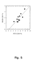
- Figure 5 plots average absolute MR versus PET values of CBV for corresponding slices under normo-and hypercapnia in 6 pigs. Care was taken to include brain parenchyma rather than large vessels in the image. Also shown is the linear regression line with slope 0.45 ⁇ 0.11 (SD) and y intercept -0.56 ⁇ 0.61(SD). Notice the apparent linearity between vascular volume measurements with PET and MRI. As both MR and PET CBV values are now in absolute values, the plot shows that only 40% of the total vascular volume is detected by the spin echo EPI MR technique.
- comparing MRI with PET may have affected our regression results in several ways.
- Co-registration of MRI and PET data may not be completely accurate, just as MR images obtained with echo planar imaging can be somewhat distorted due to magnetic field inhomogeneities and susceptibility artifacts. The latter causes anatomical structures imaged by the EPI sequence not to be imaged in the exact location as in the 3D image sequence used for co-registration.
- a more complex problem was caused by the differences in inherent resolutions of PET and MRI.
- the effective resolution with the parameters used is approximately 4.5 mm in the center of the investigated volume.
- the measurements provide insight into the selectivity for the effect of small vessels of the T 2 -weighted spin echo EPI sequence used in our experiment.
- Weisskoff et al. (1994) previously demonstrated that the susceptibility contrast in this imaging sequence arises mainly in small, capillary size vessels.
- the distribution of fractional vascular volume as a function of vascular diameter is not fully known, it is difficult to predict absolute volume values based on these simulations.
- Our 40-50% estimate of the vascular fraction detected by MR is therefore difficult to compare to theoretical predictions.
- CBF cerebral blood flow
- PET positron emission tomography
- CBF cerebral blood flow
- MRI dynamic magnetic resonance imaging
- PET positron emission tomography
- C t (t) F t ⁇ C a ( t ) ⁇ R ( t )
- ⁇ denotes the convolution of R(t), the vascular residue function (normalised impulse response function) with the arterial input function, C a (t).
- R(t) and CBF can be determined with good accuracy, independent of the underlying vascular structure and volume ( ⁇ stergaard et al., 1996a).
- the volunteers were studied in a Siemens ECAT EXACT HR PET camera using a custom-made head-holding device.
- a fast i.v. bolus injection of 500 MBq H 2 15 O in 5 ml saline was performed, followed immediately by an i.v. injection of 10 ml of isotonic saline to flush the catheter.
- a sequence of nineteen (12, 6 and 3 samples during the first, second and third minute, respectively) arterial blood samples (1 - 2 ml) and 12 PET brain images (6, 4 and 2 images per minute, respectively) were then obtained.
- Brain image data were reconstructed using scatter correction, and a Hann filter with a cutoff frequency of 0.5 pixel -1 , resulting in an isotropic spatial resolution (FWHM) of 4.6 mm.
- Correction for tissue attenuation was based on a 68 Ga transmission scan. Radioactivity levels in image and arterial blood were corrected for the half-life of 15 O (123 s).
- 15 O 2 was produced by the 14 N(d,n) 15 O nuclear reaction by the bombardment of nitrogen gas with 8.4 MeV deuterons using a GE PETtrace 200 cyclotron. 15 O 2 was mixed with hydrogen and passed in a stream of nitrogen gas over a palladium catalyst at 150°C to produce 15 O-water vapour, which was trapped in 10 ml sterile saline.
- MR imaging was performed using a GE Signa 1.0 Tesla imager (GE Medical Systems, Milwaukee, Wisconsin). Following a sagittal scout, a T 1 weighted 3D image was acquired for co-registration of MR and PET data.
- SE spin echo
- EPI echo planar imaging
- the integrated area of the arterial input curve was in each measurement normalised to the injected contrast dose (in mmol per kg body weight) according to our earlier approach ( ⁇ stergaard et al., 1997).
- Deconvolution was performed following the application of a 3x3 uniform smoothing kernel to the raw image data, and the maximum point on the deconvolved impulse response curve was chosen to be CBF.
- the 3D PET CBF images were used to automatically co-registered with the 3D MR images (Collins et al., 1994).
- Raw PET image data were then transformed and re-sampled to the same spatial location and resolution as the MR CBF data to allow direct comparison of the two techniques.
- a 3x3 uniform smoothing kernel was applied to our raw PET image data, these were fitted to equation 2 using non-linear, least squared regression analysis on a pixel-by-pixel basis.
- Pixel by pixel maps of CBF (at similar anatomical locations, pixel size and resolution) generated by PET and MR, respectively, were then compared on a regional basis. In each image, 20-25 regions of similar size were chosen, including gray and white matter. The means of all regional values were then averaged, to yield a common conversion factor between MRI flow units and absolute flow in ml/100ml/min). Regional average CBF values and their standard deviations (derived from the population of pixels within the ROI) were then compared.
- Table 3 shows values of P a CO 2 and P a O 2 for all volunteers during MR and PET measurements. Volunteer 3 showed a 13% change in P a CO 2 and was excluded from the analysis, while volunteer 1 had to be excluded due to head motion during the MR measurements.
- Figure 6 shows parametric CBF maps determined by PET and NMR, respectively. To facilitate visual comparison, the MR flow image was blurred to the resolution of the PET image. Also shown is the corresponding anatomical MR image. It is noticed that vessels appear to be treated somewhat differently by the two methods: In the PET images, these appear as high flow areas, whereas in the MR images, arterial branches appear as high flow regions.
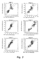
- Figure 6 shows MR versus PET plots of regional CBF values along with their standard deviations for the six volunteers. Also shown are linear regression lines and their 95% confidence regions. White matter ROIs are represented in the lower left quadrant of the plots, whereas gray matter ROIs are in the upper right.
- Figure 8 shows what may reflect a methodological problem of the MR technique.
- the MR technique is sensitive to large delays in tracer arrival, causing CBF to be somewhat underestimated.
- the tracer arrival in the posterior circulation was delayed by several seconds relative to the remaining brain. This, apart from possible differences in visual activity during the two measurements, may explain the occipital hypoperfusion in this volunteer.
- the assumption that the area under the arterial concentration time curve is proportional to the injected dose in all subjects may not hold true under all circumstances.
- circulatory disturbances may cause the characteristic time scale of the arterial input to become longer than that of the vascular transit time, making CBF measurements difficult (Kent et al 1997).
- CBF cerebral blood flow
- MR magnetic resonance
- SVD singular value decomposition
- the model-free SVD method offers the advantage of being independent of the underlying vascular structure, the method is somewhat susceptible to dispersion and delay of the measured AIF before it reaches the imaging pixel ( ⁇ stergaard 1996b).
- dispersion in the feeding vessel may be significant relative to tissue tracer retention, causing underestimation of CBF, and therefore overestimation of the CBV:CBF ratio ( ⁇ stergaard 1996b).
- This ratio, the plasma mean transit time (MTT) is an important parameter in evaluating cerebrovascular perfusion reserve, and therefore the inability of the SVD approach to distinguish vascular dispersion from prolonged tissue MTT may ultimately impair its clinical use.
- Bassingthwaighte and co-workers have developed modelling tools to describe major vessel transport as well as microvascular tracer retention (King 1993; King 1996).
- a derived model of the coronary circulation has been successfully applied to MR data, allowing non-invasive measurements of coronary blood flow (Kroll 1996).
- This model (hereafter referred to as the vascular model), modified for the cerebral circulation, may ultimately provide estimates of CBF and MTT independent of major vessel delay and dispersion.
- the aim of this study was to extend this vascular model to the cerebral circulation.
- a first-order expression of flow heterogeneity in the cerebral circulation was derived by a model-free analysis of tracer retention in areas of negligible major vessel dispersion.
- the vascular model was fitted with measured flow heterogeneity, to human MR residue measurements, and compare the resulting flow rates to literature values, as well as the SVD method. Finally, the sensitivity of the vascular model to tracer delays was compared in simulated data.
- a modified version of the vascular model previously described by Kroll et al was used.
- the vasculature was modelled a major, feeding artery in series with 20 small vessels in parallel - See Figure 10.
- the flow is directed along the parallel pathways, with w i representing the fraction of flows with values f i -Fp, where F p is total flow.
- the capillaries were modelled as simple delay lines of fixed length (100 ⁇ m), with volume Vp.
- the tissue flow F p , the feeding vascular volume V art , and capillary volume Vp was allowed to vary.
- the observed signal changes due to magnetic susceptibility contrast agent arises - when using a spin echo sequence (See Materials and Methods below) - mainly from capillaries (Fisel 1991; Boxerman 1995; Weisskoff 1994).
- total tissue tracer concentrations were therefore calculated based on the amount of tracer in the small, parallel vessels.
- the distribution of transit times in the capillary bed was incorporated by an algorithm assigning appropriate flows and weights to the parallel vascular paths, to achieve a given heterogeneity (King 1996).
- the impulse response to a plasma tracer can be estimated by nonparametric deconvolution of the tissue residue during the tracer passage by a non-invasively determined arterial input function (AIF) is utilised. From this the distribution of plasma transit times, and - under certain assumptions regarding the distribution of capillary lengths - the distribution of flows in the region are derived.
- the tissue concentration C t (t) of tracer in response to an arterial input function C a (t) is given in Equation 4.
- the formula is equivalent to the integral where F t is tissue flow and R is the residue function, i.e. the fraction of tracer present in the vasculature at time t after a perfect, infinitely sharp input in the feeding vessel.
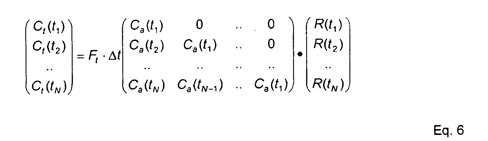
- Equation 6 Assuming the arterial and cerebral concentrations are measured at equally spaced time-points t 1 ,t 2 ,...,t N , this equation can be discretized, assuming that over short time intervals ⁇ t, the residue function and arterial input values are constant in time: which is equal to the expression in Equation 6. As previously described ( ⁇ stergaard 1996b), this equation can be modified to residue and arterial input functions that vary linearily in time. The SVD approach provides a powerful numerical tool to solve Equation 6 in the presence of experimental noise to yield the residue function. The distribution of transit times, h(t), is then found from i.e. the slope of the residue function. At a given time point t i , h(t) can be estimated as
- PDF probability density function
- Tissue concentration time curves were formed using Equation 1. Three gray and two white matter tissue regions consisting of 4 image pixels (0.05 cc) were then chosen, based on cerebral blood volume maps (Rosen 1990). The tissue residue function was calculated by SVD deconvolution of the tissue concentration time curve with the AIF. The resulting residue function was then converted into a probability density function (PDF) of relative flows as described in the Theory section above
- each pixel tissue concentration time curve was delayed in steps of 0.25 second by linear interpolation to simulate the effects of tracer arrival delays.
- the simulated image data were then analysed as described above, and fitted flow rates by the SVD and vascular model approach plotted as a function of delay for comparison.
- Simulated SNRs varied from 400 down to 12, the latter being typical for raw, pixel-by-pixel data obtained with perfusion protocols on a clinical MR system.
- 24 simulations were performed, and the mean and standard deviations of the fitted model parameters were calculated for further evaluation.
- the dependency on initial conditions was evaluated by recording the number of simulations where two different initial conditions caused resulting fitted parameters to differ by more than 10% from their mean.
- flow rates were determined from the same synthetic curves by the SVD method.
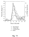
- FIG 11 shows a set of typical tissue and arterial concentration time curves obtained from volunteer 1.
- the tissue ROls consisted of 25-35 pixels (corresponding to 0.3 - 0.4 cc volumes).
- the average signal to noise ratio (SNR) (defined as the maximum tissue R 2 increase during bolus passage divided by the standard deviation of the noise relative to pre-bolus base-line image intensity) for the tissue volumes used for model validation (0.25-0.4 cc) was 30.
- the SNR of gray matter was a factor of 2 to 3 higher than that of white matter, due to the higher blood volume.
- Figure 12 shows the location and size of three regions chosen for determination of flow heterogeneity in volunteer 4.
- the regions are overlaid on a CBF map calculated by the SVD-method to illustrate the contrast and spatial resolution of the techniques.
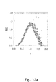
- Figure 13a shows all pairs of relative transit time t and corresponding h(t) measured for all regions in all 6 volunteers.
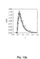
- Figure 13b shows - under the assumption of equal capillary lengths - the corresponding plot of relative flow f and w(f) measured for all regions and volunteers.
- the quality of model fits to experimental data shown in Figure 14 is typical for the patients examined. Table 5 shows the mean gray:white matter flow ratios for 8 regions.
- the mean gray:white flow ratio was 2.89 ⁇ 0.35 with the vascular model.
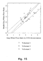
- Figure 15 shows gray:white matter flow ratios determined by the model approach plotted versus corresponding ratios in identical regions determined by the SVD approach.
- the three volunteers were chosen based on a significant spread in individual, regional gray:white matter ratios, in order to facilitate comparison between approaches.
- the line of identity was within the 95% confidence intervals of a common linear fit. Notice regional gray:white matter ratios using the two techniques all lie near the line of identity.
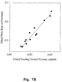
- Figure 16a shows the effect of AIF delay on fitted flow rates for the vascular model and the SVD approach, respectively.
- the gray and white matter tissue ROls consisted of 90 image pixels (1.1 cc).
- Vascular model and SVD values were obtained from identical regions.
- the SVD approach progressively underestimates flow rates with tracer arrival delay.
- the relative underestimation is roughly proportional to the delay, reaching 25% for white matter and 35% for gray matter at a delay of 3 seconds, respectively.
- flow estimates are remarkably independent of delay.
- Figure 16b shows the fitted feeding artery volume as a function of delay.
- the vascular model interprets increasing delays as increased feeding vessel volume in accordance with the definition of the vascular operator.
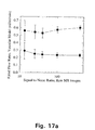
- Raw image data noise was varied from that of typical, clinical data (-12) to 400.
- the SVD approach overestimates flow rates somewhat for this choice of model parameters, whereas the vascular model fits are roughly equal to the input parameters.
- the uncertainty (error bars in Figure 17a and 17b indicate one standard deviation, derived from the simulated data) on fitted flow rates display the expected increase as a function of increasing raw image data noise.
- the vascular model after incorporation of the experimentally determined heterogeneity PDF, provided excellent fits to the experimental data.
- the model fits of CBF yielded a mean gray:white flow ratio of 2.8 ⁇ 0.35, in agreement with the PET literature ratio of 2.65 for subjects of similar age (Leenders 1990). The ratios were also in good agreement with those found using the model-free approach.
- the model approach provided fits to experimental data that were essentially independent of vascular delay.
- the model was simplified considerably by the use of one flow heterogeneity PDF for all types of tissue. By characterising the model by only three parameters, a remarkable stability of the model was obtained, even compared to the pixel-by-pixel based SVD approach. Co-varying vascular volume and flow rate in model fits to low SNR data was found to be a major contributor to uncertainty in model fits of CBF. Below, the individual elements of the model are discussed in further detail.
- Kroll et al. Kroll 1996) described the arteriolar and capillary compartments separately, assigning fixed relative dispersion and variable volumes to the arteriolar vascular paths, and a fixed volume to the capillary bed.
- capillary density varies greatly among different tissue types.
- the microvascular volume was kept as a free parameter.
- the models are similar, except that in the model presented here, dispersion takes place only in the large vessel, whereas small vessel dispersion is accounted for by the flow heterogeneity PDF.
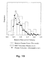
- capillary plasma flow and flow velocity is a complex function of capillary length and architecture, a finite distribution of capillary lengths is likely to result in blood velocities being more dispersed than relative capillary flows (As seen when comparing the PDF presented here with the RBC velocity study).
- the similarity of the present measurements with these independent, invasive methods lends hope to the use of this approach in describing normal microvascular dynamics.
- the flow heterogeneity may not be as constant among tissue types as found in this study.
- Abounader et al. (Abounader 1995) determined the heterogeneity of microvascular flow at different degrees of hypercapnia, and found that plasma flow became more homogenous at higher flows.
- Acute stroke is the third leading cause of death, and the leading cause of adult disability. Emerging therapeutic strategies seek to minimise the progression of tissue damage in the acute phase of the disease. Methods to rapidly assess the severity and later progression of acute stroke in individual patients are therefore highly desirable to plan individual treatment, as well as to evaluate novel therapeutic strategies.
- vasoregulatory control is believed to be the ability to alter the heterogeneity of blood transit times and thereby the mean capillary concentration of substances diffusing from blood to tissue (Kuschinsky and Paulson 1992).
- Animal experiments in rats have revealed decreased flow heterogeneity during whisker-barrel stimulation(Vogel and Kuschinsky 1996), indicating that this may be the mechanism underlying the normal brain's striking ability to meet increased metabolic needs during functional activation.
- Hudetz et al. demonstrated that graded decrease in perfusion pressure causes progressive loss of high-flow components, thereby decreasing total flow heterogeneity (Hudetz 1996).
- MRI Perfusion Protocol Determination of CBV, CBF, MTT, and flow heterogeneity. Perfusion imaging was performed using spin echo (SE) or gradient echo (GE), echo planar imaging (EPI) with a time of repetition (TR) of 1.5 seconds, and a time of echo (TE) of 100 ms (50 ms for GE EPI).
- SE spin echo
- GE gradient echo
- TE time of echo
- the slice thickness was 5 mm with an in-plane resolution of 1.56 mm by 1.56 mm in a 40 by 20 cm field-of-view (FOV). In 10 slices, a total of 52 images were acquired, starting 15 seconds before i.v. injection of 0.2 (SE-EPI) or 0.1 (GE-EPI) mmol/kg Gd-based contrast agent.
- Intravascular contrast agent concentrations were quantified assuming a linear relationship between concentration and change in transverse relaxation rate, AR 2 (Villringer 1988; Weisskoff 1994).
- the shape of the arterial input function was determined from feeding arterial branches either adjacent to the area of DWI abnormality or at the contralateral middle cerebral artery (MCA), and were, identified in the image slice as pixels displaying early concentration increase after contrast injection (Porkka 1991).
- the tissue residue function (or impulse response function) was calculated by deconvolving the tissue concentration time curve by the AIF, using singular value decomposition (SVD) ( ⁇ stergaard 1996a; ⁇ stergaard 1996b).
- CBF was determined as the height of the deconvolved tissue curve.
- CBV was determined by the area under the tissue concentration time curve, as previously described (Rosen 1990), and the plasma mean transit time (MTT) formed as the ratio CBV/CBF (Stewart 1894). Finally, the distribution of tissue transit times in each imaging voxel was determined as the slope of the residue function, and by assuming equal lengths of capillary paths, the corresponding probability density function (PDF) of relative flows was determined by means of the central volume theorem(Stewart 1894; Example 3 ( ⁇ stergaard 1999)).
- PDF probability density function
- infarct size was assessed by diffusion weighted imaging (DWI) (Moseley 1990), acquired using single-shot EPI (TR 6 s, TE 118 ms) with diffusion weighting applied in 6 directions.
- DWI diffusion weighted imaging
- EPI TR 6 s, TE 118 ms
- Final infarct size was assessed from DWI images acquired 2-5 days after the infarct, from T 2 or FLAIR MR images acquired at least 5 days after the infarct, or from CT images acquired more than 5 days after the infarct if no MRI was available.
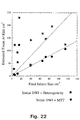
- Figures 20a, 20b, and 20c show a typical pattern in patient 6. This patient, a 64 year old female, was examined 5.5 hours after onset of left leg weakness, and showed prolonged MTT corresponding to the anterior cerebral artery territory ( Figure 20a).
- Figure 20b shows the flow heterogeneity plots for normal brain tissue as well as two regions of prolonged mean transit time (Areas are indicated on the MTT map with numbers corresponding to the PDF curves).
- the flow PDF in normal tissue was markedly right-skewed, and matched the shape previously found in normal volunteers (Example 3 ( ⁇ stergaard 1999)).
- the volumes of increased MTT displayed PDFs with a more symmetric shape, with a tendency to loose the high-flow population found in normal tissue.
- the degree of symmetry varied within the volume of increased MTT.
- the deviation from the normal PDF was subsequently quantified by a Kolmogorov-Smirnov test, yielding the probability p that the curve belong to the distribution of relative flows of normal tissue (from Example 3 ( ⁇ stergaard 1999)).
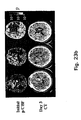
- Figures 24a and 24b show maps from patient 9, a 80 year old female. Small infarcted areas are seen on the initial DWI images (Top row). The MTT image shows abnormalities extending into white matter around the initial lesions. Again, flow heterogeneity changes are observed in smaller subregions, corresponding well to the regions that went on to infarction. Notice symmetrically located areas with low p values, corresponding to vessels.
- the findings presented hence strongly support the hypothesis by Hudetz et al that gradual loss of the high flow component of the flow heterogeneity PDF heralds local loss of functional reserve capacity, and thereby neuronal death (Hudetz 1996).
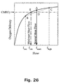
- oxygen flow into the tissue at a given mean blood flow is greater when blood flow is homogenous than when blood flow is more heterogeneous:
- Oxygen flow into tissue versus blood flow F t related through the equation F t ⁇ (1-e -PS/F t ), where PS is the permeability to oxygen times the surface area of capillaries (Renkin 1959; Crone 1963).
- F t the normal mean flow
- f norm the oxygen flow into tissue is given by the height of A. If part of the flow is at f low and the rest at f high , with weightings to maintain the same mean flow, the oxygen flow into the tissue will be the height of D.
- the AIF may undergo dispersion and delays upstream of site of measurement, possibly causing overestimation of MTT ( ⁇ stergaard 1996a; ⁇ stergaard 1996b).
- This bias was reduced by choosing AlFs in the vascular territory affected by the vascular occlusion.
- dispersion of the AIF will tend to broaden the flow PDF. Therefore, the effects of dispersion counteract the observed homogenisation of flow elements.
- high p values were observed near vessels (and therefore easily identifiable on the accompanying CBV maps), as major vessel flow inherently homogenous. Probability maps should therefore be carefully inspected for vessels on CBV maps, as well as signs of vessel dispersion in the PDF shape in a given region.
- SE-EPI images are particularly suited for this type of analysis, as large vessels are suppressed due to the inherent microvascular weighting of these images (Fisel 1991; Boxerman 1995; Weisskoff 1994).
- Noninvasive methods for assessing individual renal function are essential in diagnosis of disease as well as in subsequent monitoring of disease progression, especially the deterioration of renal function in renal artery stenosis, diabetes, ureteral obstruction, neurogenic bladder, and to identify rejection or other postoperative complications in renal transplants.
- the questions often asked is whether function is stable or deteriorating, thereby detecting changes at early stages where treatment may still be possible, or in some cases in unilateral disease to determine whether the patient may benefit from nephrectomy.
- Unilateral renal function is today almost exclusively determined by radionucleide measurements, using mostly 99m Tc, 51 Cr or 131 I/ 1233 I bound agents and gamma camera detection.
- the radiotracers fall into three main groups, filtered agents that are exclusively filtered in the glomeruli, secreted agents that are totally removed from the blood into the urine during a single transit, and finally the more rare bound agents which display some degree of binding to the renal parenchyma.
- Filtered agents mainly 99m Tc-DTPA
- GFR glomerular filtration rate
- Secreted agents e.g. 99m TC-MAG 3 , 123 I/ 131 I-OIH
- RPF renal plasma flow
- Bound agents e.g. 99m Tc-DMSA, 99m Tc-GHA
- these agents would show regional uptake in the parenchyma proportional to tissue flow.
- the functional indices derivable from dynamic images acquired after injection of these agents are closely related to the characteristic transport and uptake over time.
- the early phase ( ⁇ 1 minute) after the injection of either filtered or secreted agent mainly display the initial, vascular distribution of the tracer and is referred to as the vascular transit segment. This phase is to some extent related to renal blood flow, as a rapid transit presumably signal high blood flow.
- the nephron transit segment ( ⁇ 1-5 minutes, i.e. uptake/transport through the nepron) reflects GFR for a filtrated agent and RPF for a secreted agent.
- the body transit segment (10-30 minutes) detects either clearance of tracer from the whole body or the appearance of tracer in the bladder. Again, by the properties of the tracer, the rate of clearance reflects RPF for secreted agents and GFR for filtered agents
- Contrast enhanced MR imaging using Gd-chelates such as Gd-DTPA provide a complete analogue to 99m Tc-DTPA renography for GFR measurements, but offering superior spatial resolution and the advantage of being free of exposure to ionizing radiation.
- these GFR measurements can be supplemented by high resolution haemodynamic information.
- novel developments in characterizing microscopic flow- and transit time heterogeneity may allow addressing the regional microscopic haemodynamics, thereby possibly improving diagnostic power of non-invasive tomographic techniques.
- Dynamic images were acqired using a Fast Field Echo (FFE) with a repetition time (TR) of 11.3 ms, echo time (TE) 8.0 ms and a flip angle of 12°. Dynamic images could hence be acquired once every 1.2 second.
- Image Field Of View (FOV) was 280 by 280 mm with a 256 by 256 resolution, leading to an in-plane resolution of 1.09 mm 1.09 mm at a 6 mm slice thickness.
- a series of 60 dynamic images were acquired during the rapid bolus injection of 1 mg Fe/kg of NC100150, an ultra small iron oxide particle (USPIO) intravascular contrast agent (Nycomed-Amersham, Oslo, Norway). Experimental data are courtesy of Lars Johannson and Atle Bj ⁇ rnerud, Nycomed Imaging AS.
- tissue impulse response to a plasma tracer can be estimated by non-parametric deconvolution of the tissue residue during the tracer passage by a non-invasively determined AIF. From this we derive the distribution of plasma transit times.
- the tissue concentration C t (t) of tracer in response to an arterial input function C a (t) is given by where F is tissue flow and R is the residue function, i.e. the fraction of tracer present in the vasculature at time t after a perfect, infinitely sharp input in the feeding vessel.
- this equation can be modified to residue and arterial input functions varying linearly in time, and solved by Singular Value Decomposition (SVD) to yield the residue function.
- Singular Value Decomposition Singular Value Decomposition
- Tissue concentrations were estimated assuming the concentration at time t, C t (t), is proportional to the change in transverse relaxation rate, i.e. where S(t 0 ) is the baseline signal intensity, S(t) the signal intensity at time t and TE the echo time (k is here a constant depending on the contrast agent and the blood characteristics). Arterial concentrations were obtained in a similar manner, from pixels located at the renal artery in the hilus region.
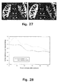
- Figure 27 shows typical parametric renal flow images acquired, immediately after and 105 minutes after ureteral occlusion. Note the high spatial resolution (1.09 by 1.09 mm) compared to the roughly 10 by 10 mm resolution of most radionucleide scans. Also note high contrast over surrounding muscle tissue displaying much lower plasma flow. Generally, little problems due to motion during the dynamic imaging session was experienced. In Fig. 27 is shown images showing high resolution images of relative renal plasma flow 15 minutes after (left) and 105 minutes after (right) obstruction of the left ureter (located at right hand side in the images). Notice the dilation of the left kidney and marked reduction in flow after obstruction
- Figure 28 shows the temporal evolution of renal plasma flow and volume after ureteral occlusion. Notice the gradual and parallel decrease in both quantities after occlusion, reaching 20% after 100 minutes. The plasma volume displays a short increase immediately after occlusion, seemingly keeping plasma flow at constant values.
- Fig. 28 is shown temporal evolution of renal plasma flow and volume after ureteral occlusion.
- Whole kidney parenchyma was manually segmented by an image analysis program (Cheshire, Hayden, Boulder, CO).
- a similar Region Of Interest could be used for all time points, but for the occluded side, ROI's had to be adjusted to take dilation into account.
- the occluded kidney values were then normalized to the contralateral side. Notice the gradual and parallel decrease in both quantities after occlusion, reaching 20% after 100 minutes.
- the plasma volume displays a short increase immediately after occlusion, seemingly keeping plasma flow at constant values.
- Figure 29 shows transit time characteristics measured as the averaged transport functions in 4 pixels from to regions.
- normalized transport functions were of similar shape.
- Only the tissue at the base of the pyramids showed a slightly more homogenous transit time distribution.
- Transit times were of the order of 1 second, and relatively uniform across the kidneys. No differences between kidneys were observed in the transit time distributions in ureteral obstruction.
- Fig. 29 is shown distribution of transit times relative to the mean transit time.
- the shape of the distribution was very homogenous across the paranchyma (full line): One exception was noticed in the pyramids (Dashed line) with a slightly more homogenous distribution of transit times. We speculate this may be due to a fraction of the vessels being vasa recta in this ROI.
- These ROIs may display a more homogenous flow distribution due to the difference in capillary organization in pyramids relative to cortical areas.
- Tumor growth is limited by the neoplasms ability to stimulate surrounding tissue to form new vessels.
- Tumour angiogenesis by release of humoral factors (Vacular endothelial growth factor - VEGF) is thereby one of the hallmarks of tumour growth, and also constitutes the target of novel approaches to treat human neoplasms.
- Methods to non-invasively assess the size, density and integrity of tumour microvessels are therefore essential to detect malignancies, understand tumour growth, and to target and monitor new therapeutic approaches (Ferrara and Alitalo, 1999).
- Dynamic susceptibility contrast imaging measuring cerebral blood volume (CBV), has for some time been used to characterise cerebral haemodynamics (Rosen et al., 1990; Rosen et al., 1991a; Rosen et al., 1991 b). Together with the specific sensitivity of spin echo (SE) Echo Planar Imaging (EPI) (Weisskoff et al., 1994; Boxerman et al., 1995) to microvessels, this approach provides a unique potential to study the proliferation of capillary sized vessels in tumour angiogenesis. As the ability to form new vessels is closely related to the growth potential and thereby aggressiveness of the tumour, the relation between histological tumour grade and regional CBV has been studied extensively. Aronen et al.
- Cerebral blood flow (CBF), CBV and flow heterogeneity was determined on a pixel by pixel basis as previously described ( ⁇ stergaard et al., 1999a; ⁇ stergaard et al., 2000).
- the distribution of flows was compared to that of normal brain by a Kolmogorov Smirnov test to identify areas of abnormal flow distributions ( ⁇ stergaard et al., 2000)
- Figure 30 shows structural T 2 -weighted image (left) of a female with a grade II astrocytoma, showing edema in the medial part of the left parietal lobe.
- the image of relative CBV (middle) shows areas of high CBV (arrow) in the centre of the tumour process, indicating angiogenic activity.
- the image at the right shows areas of abnormal distribution of flows compared with normal brain tissue ( ⁇ stergaard et al., 1999a) as coloured areas overlayed onto the CBV map. Notice that within the tumour process, areas showing highly heterogeneous flow distributions are found, likely due to the increased tortuosity of the newly formed vessels.
- Fig. 30 shows structural T 2 -weighted image (left) of a female with a grade II astrocytoma, showing edema in the medial part of the left parietal lobe.
- the image of relative CBV (middle) shows areas of high CBV (arrow) in the centre of the tumour process, indicating angiogenic activity.
- the image at the right shows areas of abnormal distribution of flows compared with normal brain tissue ( ⁇ stergaard et al., 1999a) as coloured areas overlayed onto the CBV map. Notice that within the tumour process, areas showing highly heterogeneous flow distributions are found, likely due to the increased tortuosity of the newly formed vessels.
Landscapes
- Health & Medical Sciences (AREA)
- Life Sciences & Earth Sciences (AREA)
- Engineering & Computer Science (AREA)
- Physics & Mathematics (AREA)
- Nuclear Medicine, Radiotherapy & Molecular Imaging (AREA)
- Medical Informatics (AREA)
- Radiology & Medical Imaging (AREA)
- General Health & Medical Sciences (AREA)
- High Energy & Nuclear Physics (AREA)
- Public Health (AREA)
- Heart & Thoracic Surgery (AREA)
- Biomedical Technology (AREA)
- Molecular Biology (AREA)
- Surgery (AREA)
- Animal Behavior & Ethology (AREA)
- Pathology (AREA)
- Biophysics (AREA)
- Veterinary Medicine (AREA)
- General Physics & Mathematics (AREA)
- Dentistry (AREA)
- Optics & Photonics (AREA)
- Oral & Maxillofacial Surgery (AREA)
- Signal Processing (AREA)
- Condensed Matter Physics & Semiconductors (AREA)
- Computer Vision & Pattern Recognition (AREA)
- Theoretical Computer Science (AREA)
- Quality & Reliability (AREA)
- Magnetic Resonance Imaging Apparatus (AREA)
- Ultra Sonic Daignosis Equipment (AREA)
- Apparatus For Radiation Diagnosis (AREA)
- Image Processing (AREA)
- Measuring Pulse, Heart Rate, Blood Pressure Or Blood Flow (AREA)
Abstract
Description
So far, the measurement of flow heterogeneity has been limited to the study to superficial vessels in the cortex of anaesthetised animals by high-speed intravital microscopy. There are no pre-existing tools that allow determination flow heterogeneity in deeper structures, or on humans as part of non-invasive, routine diagnostic procedures.
determining the impulse response function of the organ or of the part of tissue by deconvolution of the time series of tomographic data with the time series of concentration data,
determining the relative tissue flow from the impulse response function of the organ or of the part of tissue,
normalising said time series of concentration data with the integral of said time series of concentration data with respect to time,
determining the normalised relative tissue flow, respectively the normalised blood volume, of the organ or part of tissue by use of the relative tissue flow and the time series of normalised concentration data, and
converting said normalised relative tissue flow, respectively normalised blood volume, to an absolute value for the tissue flow, respectively the blood volume, by means of a previously determined conversion factor,
the quantitative haemodynamic parameter being of metabolic significance and determined from the PDF and the absolute tissue flow, respectively the absolute blood volume.
where the random formation of irregular vessels causes increased heterogeneity of flows and transit times due to the passage through irregular vascular paths. (b) Vasculopathies, i.e. diseases where normal vascular wall architecture is disrupted, altering the passage and thereby flow heterogeneity of blood or tracer molecules, such as collagen vascular diseases (Systemic lupus erythematosus, rheumatoid arthritis, other connective tissue disorders), vasculitis (giant cell arteriritis, polymylagia rheumatica), micro- and macroangiopathies in diabetes, angiopathy due to hypertension. (c) Changes in vascular architecture due to chronic or degenerative processes of organs (liver, kidneys, heart, brain) in general. In particular the method may be used in connection with assessment of disease stage (e.g. tumor grade, extent of abnormal tone in renal afferent arterioles in hypertension or acute renal failure, extent of change in glomerular capillary structure in degenerative renal diseases) based on heterogeneity measurements, evaluation of drug efficacy in these diseases based on quantification of heterogeneity measurements (e.g. anti-angiogenic treatment), and planning treatment based on prior knowledge of flow or transit time heterogeneity and the associated risk of amelioration of disease.
In connection with organ transplantations it is generally of great value to know the vascular supply and the capacity of the vascular system of the organ.
Furthermore, the method determines the distribution of flow and mean transit time, either in absolute values or relative to the mean value. The methods further allows the (i) comparison of relative flow distributions to that of normal tissue (here brain) or (ii) quantification of absolute flow distributions in terms of the associated extraction of a substance with known capillary permeability.
normalisation of the arterial input area to the injected dose of contrast agent per kg body weight.



Here, relative flow, Fr, means a value proportional to (by the same factor throughout the digitised images of relative flows) absolute flow in cases where absolute arterial flow values cannot be determined. Again, absolute flow refers to cases where arterial concentrations are known in the units of the tissue concentration data.
where absolute arterial flow values cannot be determined. As above, an absolute flow refers to the cases where arterial concentrations are known in the units of the tissue data.
CBF = 0.87· Bo· F r (humans)
CBV = 0.87· Bo· V r (humans)
CBF = 1.09· Bo. Fr (porcine data)
CBV = 1.09· Bo· Vr (porcine data)
Where Bo is the field strength of the magnet in Tesla, and Vr and Fr are the relative volumes and flows determined as described in
Special cases:

| f | w(f) | f | w(f) |
| 3.8053 | 1.65E-03 | 0.6941 | 1.4594 |
| 2.865 | 0.0226 | 0.647 | 1.5915 |
| 2.3306 | 0.0372 | 0.6205 | 1.6279 |
| 1.7879 | 0.0627 | 0.5969 | 1.5812 |
| 1.5881 | 0.1198 | 0.5815 | 1.351 |
| 1.4459 | 0.1751 | 0.565 | 1.3393 |
| 1.3535 | 0.2491 | 0.5448 | 1.2367 |
| 1.2785 | 0.3303 | 0.5262 | 1.1433 |
| 1.1912 | 0.4058 | 0.5133 | 1.0688 |
| 1.1106 | 0.4793 | 0.5007 | 0.928 |
| 1.0474 | 0.646 | 0.4822 | 0.6559 |
| 0.9972 | 0.7218 | 0.4689 | 0.6366 |
| 0.9438 | 0.9032 | 0.4571 | 0.4282 |
| 0.8981 | 0.986 | 0.4416 | 0.3133 |
| 0.8214 | 1.1098 | 0.4316 | 0.0244 |
| 0.7794 | 1.3562 | 0.42 | 0 |

With regard to cerebral blood flow (CBF) determined from contrast bolus passage, there has been uncertainty whether CBF can be measured reliably with MRI, due to inherent theoretical problems (Lassen, 1984; Weisskoff, 1993). Recent results indicate that MRI can be used to measure CBF, in that mean gray:white matter flow ratios measured by dynamic spin echo (SE) echo planar imaging (EPI) in normal humans were similar to PET literature ratios for CBF for age-matched subjects (Østergaard et al. 1996a; 0stergaard et al 1996b). The bolus technique has only been able to yield relative CBF values within a given subject. In this report, we present a procedure for determining absolute CBF values by means of MRI. We compared the CBF values to the results of the PET [15O] water clearance method in hypercapnic animals. We also studied the microvascular sensitivity of MRI CBV measurements, comparing quantitative CBV measured with MRI by our approach, and PET [15O]CO estimates of vascular volume.


In all experiments, bolus injection of 0.2 mmol/kg Gadodiamide (OMNISCAN® , Nycomed Imaging, Oslo, Norway) was performed manually at a rate of 15-20 ml/s. Prior to the first dose, a pre-dose of 0.05 mmol/kg was given to avoid systematic effects from changes in blood T1.

The arterial concentration was determined in each animal from pixels containing large, feeding vessels (typically the middle cerebral artery) showing an early and large (3-10 times that of gray and white matter) increase in Δ R2 following contrast injection. This method has previously been demonstrated to closely reflect actual, arterial levels for the susceptibility contrast agents used in this study when imaged using spin echo EPI techniques (Porkka et al., 1991). The integrated area of the arterial input curve was in each measurement normalised to the injected contrast dose (in mM per kg body weight) in order to compare within and among animals.
To determine CBF from equation 12, the deconvolution was performed over the range of measurements where the arterial input values exceeded the noise level (usually about 15 seconds). Deconvolution followed smoothing of raw image data by a 3 x 3 uniform smoothing kernel to. The maximum of the deconvolved response curve was assumed proportional to CBF. CBV was determined by numerically integrating the concentration time curve from bolus arrival to tracer re-circulation.
The two constants a and b were determined for each pixel, and CBV and CBF were corrected.
Figure 1 shows parametric maps of CBF for pig no. 4. The pixel size is the same in the two images. Notice the good overall agreement between the regional values and responses to arterial CO2 levels using the two methods, although the MRI CBF map appears to distinguish better between gray and white matter structures than the PET CBF maps. Notice also that the PET CBF map appears to be somewhat noisier than the MRI CBF map. We investigated possible regional differences in CBF maps obtained by the two methods. These appeared to be mainly associated with either noise artifacts or the presence of veins in the PET image slice. Noise in PET images appears as 'streaky artifacts' that sometimes propagate into the CBF maps. Veins, on the other hand, are often interpreted by the kinetic model in equation 13 as a high flow region, whereas they are rarely detected by the MR sequence.
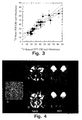
Figure 2 shows plots of regional CBF values with their standard deviations for individual pigs. Notice that normo- as well as hypercapnic data points are plotted in the same diagram to visualize overall agreement of absolute values as well as responses to CO2 among PET and MRI. There was a tendency for normocapnic data points to be grouped in the lower left and hypercapnic data points in the upper right quadrant of the plots. Notice that the error bars associated with the MRI measurements appear smaller than the corresponding PET values for the same region. The average standard deviation on regional flow estimates was on the average 30% smaller than the corresponding standard deviation for the same PET ROI. Figure 3 shows the corresponding plot for repeated PET measurement of CBF with 15O butanol. The results of the linear regression analysis are shown in Table 2. The slopes of the linear regression lines did not significantly differ among the pigs (by multiple pairwise t-tests). For most animals, the regression coefficient r2 (the proportion of the variance accounted for by the regression) ranged between 0.7 and 0.8.
| Pig | a | | r | 2 |
| 1 | 0.82±0.10 | 11±5 | 0.79 | |
| 2 | 1.00±0.11 | -2±6 | 0.81 | |
| 3 | 0.99±0.15 | 0±10 | 0.70 | |
| 4 | 0.97±0.11 | -4±6 | 0.79 | |
| 5 | 0.98±0.11 | 2±7 | 0.81 | |
| 6 | 0.90±0.12 | 6±5 | 0.75 | |
| 6* | 0.77±0.07 | 10±3 | 0.86 |
First, assuming a common constant that relates injected MR contrast dose to the area under the image-based arterial input concentration time curve may not always hold true. The validity of this assumption is sensitive to the fraction of the injected contrast dose delivered to the brain circulation in the two experimental conditions, and more importantly, the linearity between contrast concentration and change in transverse relaxation rate assumed in
As for more methodological problems, comparing MRI with PET may have affected our regression results in several ways. Co-registration of MRI and PET data may not be completely accurate, just as MR images obtained with echo planar imaging can be somewhat distorted due to magnetic field inhomogeneities and susceptibility artifacts. The latter causes anatomical structures imaged by the EPI sequence not to be imaged in the exact location as in the 3D image sequence used for co-registration. In cases where we noticed slight in-plane differences in locations, we adjusted the location of the ROI in the MRI images to account for this fact.
A more complex problem was caused by the differences in inherent resolutions of PET and MRI. For our PET tomograph, the effective resolution with the parameters used is approximately 4.5 mm in the center of the investigated volume. By using a Gaussian filter, we sought to blur the MRI measurements to yield the same resolution as the PET CBF measurements. However, the CBF images in Figure 1 still indicate that there may be differences in resolution that are not accounted for, causing influence from neighbouring regions to be different in the two imaging modalities, thereby causing a non-linear relationship between regional CBF values simply due to differences in resolution. We believe these factors explain the slightly better regression statistics obtained when comparing two PET CBF measurements rather than comparing MR.
The measurements provide insight into the selectivity for the effect of small vessels of the T2-weighted spin echo EPI sequence used in our experiment. By a Monte Carlo simulation approach, Weisskoff et al. (1994) previously demonstrated that the susceptibility contrast in this imaging sequence arises mainly in small, capillary size vessels. As the distribution of fractional vascular volume as a function of vascular diameter is not fully known, it is difficult to predict absolute volume values based on these simulations. Our 40-50% estimate of the vascular fraction detected by MR is therefore difficult to compare to theoretical predictions. However, studies of peripheral tissue indicate that vessels smaller than 30-40 µm diameter (small arteries, arterioles, capillaries, venules and small veins) represent roughly 50% of the total vascular volume (Johnson, 1973). Assuming that the MR measurements are predominantly sensitive to the smallest vessels, our value of 40-50% therefore points towards a sensitivity to vessels smaller than 30-40 µm of the MR technique. This in turn makes the CBF and CBV techniques sensitive to microvascular phenomenons, e.g. neovascularization in neoplasia (Aronen et al., 1994) and flow-volume mismatches in stroke due to delayed passage through oxygen exchanging vessels (Heiss et al. 1994).
In this study we compare absolute regional NMR bolus CBF values with CBF values determined by [15O] water uptake, detected by positron emission tomography (PET) in normal human volunteers.
It has been demonstrated that, using singular value decomposition (SVD), R(t) and CBF can be determined with good accuracy, independent of the underlying vascular structure and volume (Østergaard et al., 1996a).


| Subject | PaCO2 (kPa) | PaO2 (kPa) | |||||
| no | PET | MR | % change | PET | | % change | |
| 1 | 5.97 | 5.63 | -5.7 | 12.11 | 13.45 | 4.8 | |
| 2 | 5.49 | 5.35 | -2.5 | 15.815 | 16.395 | 3.7 | |
| 3 | 6.63 | 5.79 | -12.7 | 12.05 | 12.625 | 4.8 | |
| 4 | 5.31 | 5.33 | 0.4 | 15.58 | 16.165 | 3.8 | |
| 5 | 5.25 | 5.325 | 1.4 | 17.175 | 15.265 | -11 | |
| 6 | 4.92 | 4.93 | 0.2 | 15.165 | 14.67 | -3 | |
| 7 | 4.485 | 4.675 | 4.2 | 15.925 | 16.97 | 6.6 | |
| 8 | 4.965 | 4.965 | 0 | 16.16 | 15.205 | -5.9 |
Figure 6 shows parametric CBF maps determined by PET and NMR, respectively. To facilitate visual comparison, the MR flow image was blurred to the resolution of the PET image. Also shown is the corresponding anatomical MR image. It is noticed that vessels appear to be treated somewhat differently by the two methods: In the PET images, these appear as high flow areas, whereas in the MR images, arterial branches appear as high flow regions. Figure 6 shows MR versus PET plots of regional CBF values along with their standard deviations for the six volunteers. Also shown are linear regression lines and their 95% confidence regions. White matter ROIs are represented in the lower left quadrant of the plots, whereas gray matter ROIs are in the upper right. There was no systematic deviation from the regression lines for gray and white matter flow rates, in agreement with the qualitative appearance of the flow maps in Figure 6. Also, notice that error bars are of comparable size for PET and MR for identical size ROIs. Table 4 shows the regression results. The portion of the variance accounted for by the regression (r2), was generally between 65 and 83 percent (see Table 4). To test whether the differences in regression slopes could be ascribed to individual uncertainties, the F statistic was calculated, showing no significant differences. Still, it was noticed that subject 5 had a somewhat larger slope than the remaining volunteers. In one volunteer (subject 8), we found an apparent hypoperfusion in the occipital lobe not visible in the PET CBF image (Figure 8). We will discuss the implications of this below.
| Subject | Slope (mi±si) | | r | 2 |
| 2 | 1.09±0.17 | 6.88±5.17 | 0.65 | |
| 4 | 1.08±0.14 | -0.48±3.58 | 0.77 | |
| 5 | 1.34±0.17 | -6.84±4.21 | 0.74 | |
| 6 | 1.01±0.10 | -10.86±5.92 | 0.83 | |
| 7 | 1.12±0.12 | 1.73±3.29 | 0.79 | |
| 8 | 0.94±0.14 | 2.41 ±6.42 | 0.66 | |
| Mean | 1.10±0.14 | -1.19±6.51 | 0.74 |
The variance observed relative to a simple linear relationship between the two different CBF estimates can be ascribed to several factors. First, CBF measurements were performed about 2 hours apart, and even though the arterial CO2 levels were nearly identical, changes in the overall level of consciousness may have resulted in different flow rates. Also, as regional flow is unlikely to be constant over even very short time scales, the fact that the MR CBF measurements are acquired in only 15 seconds, whereas radiolabeled water levels are observed for three minutes by PET, may contribute to differences in regional values. More technical and methodological issues may have affected our measurements, as well. First, the rapid EPI sequence used in our measurements is sensitive to magnetic field inhomogeneities. This may result in misregistration of corresponding PET and MRI regions. This is illustrated in Figure 8, displaying the conventional MRI as well as the PET CBF maps from the
There were some qualitative differences among the CBF images obtained by the two modalities. The MR technique was found to interpret small arteries as high flow regions. This is inherent to the technique, as it does not mathematically distinguish between large vessel and capillary tracer dispersion. However, as CBV is simultaneously determined by integration of the tissue concentration time curve (Rosen et al. 1991), this does not pose a problem in interpreting the CBF maps. Also, due to the inherent sensitivity of susceptibility contrast imaging to small vessels (Fisel et al. 1991, Weisskoff et al. 1994) large vessels are not seen in the images. In contrast, PET CBF images partly interpret dispersed venous blood as tissue flow, whereas arteries are suppressed by means of the Vo term in equation 17.
In one volunteer (subject 8), we found a marked hypoperfusion in the occipital lobe possibly due to delay in the arrival of tracer in the posterior circulation. This effect was predicted in theoretical simulations of the technique (Østergaard et al. 1996a). Figure 9 shows how flow estimates become increasingly underestimated as the arrival delay of the tracer at a brain region increases, in both PET and MR CBF measurements (Simulations were performed by simply introducing delays between the arterial and cerebral concentration time curves in volunteer 6). Notice, however, that whereas PET measurements may underestimate flow by 15%, underestimation by MRI can be as much as 50%. Even though we only noticed this effect in one volunteer, these simulations underline the importance of further evaluating this technique in patient populations with e.g. vascular diseases. Also, we are currently working on approaches to minimise the sensitivity of our CBF algorithm to tracer arrival delays.
We used rather low spatial resolution (64 by 64 matrix), single slice measurements. It is worth noticing that most current MR systems with EPI capabilities allows multi-slice acquisitions at a considerably higher spatial resolution (typically 2.5 by 2.5 mm pixels). This allows CBF measurements at twice the spatial resolution of most current PET systems.
The tissue concentration Ct(t) of tracer in response to an arterial input function Ca(t) is given in


As previously described (Østergaard 1996b), this equation can be modified to residue and arterial input functions that vary linearily in time. The SVD approach provides a powerful numerical tool to solve


Feeding arterial branches were identified in the image slice as pixels displaying early concentration increase after contrast injection (Porkka 1991). This approach does not determine absolute arterial tracer levels, but provides the shape of the AIF. To standardise the analysis below, the arterial input function was therefore scaled to yield a mean CBV of 3% (Example 1 (Østergaard 1998b)). In volunteers, a single arterial input function in the imaging plane was used for all tissue regions.
| Regional gray:white flow ratios in 6 volunteers | |||||||
| Volunteer no. | |||||||
| | 1 | 2 | 3 | 4 | 5 | 6 | Average |
| Basal ganglia left | 4.19 | 3.41 | 3.70 | 2.73 | 3.76 | 3.39 | 3.53 |
| right | 3.76 | 3.41 | 2.99 | 2.80 | 3.66 | 3.86 | 3.41 |
| Frontal medial left | 2.89 | 2.91 | 1.94 | 2.32 | 2.55 | 2.03 | 2.44 |
| right | 2.66 | 2.73 | 3.6 | 2.24 | 3.06 | 3.03 | 2.88 |
| Temporal left | 3.55 | 3.16 | 3.14 | 2.55 | 4.31 | 2.29 | 3.16 |
| right | 4.52 | 3.59 | 3.27 | 2.02 | 3.71 | 2.78 | 3.31 |
| Occ.-temporal left | 2.50 | 2.37 | 2.66 | 2.20 | 2.55 | 2.74 | 2.50 |
| right | 2.78 | 2.05 | 3.70 | 2.08 | 1.70 | 1.97 | 2.38 |
| Occ. medial left | 3.60 | 2.87 | 2.27 | 2.06 | 2.30 | 2.84 | 2.66 |
| right | 2.95 | 2.12 | 3.57 | 2.17 | 2.15 | 2.43 | 2.57 |
| Average | 3.34 | 2.86 | 3.08 | 2.31 | 2.97 | 2.74 | 2.89 |
Imaging was performed on a GE Signa 1.5 T imager (General Electric, Waukesha, WI) retrofitted for EPI capabilities (Instascan, Advanced NMR Systems, Wilmington, MA).
| Patient | Age/ | Hours | |
| 1 | 33 M | 4.5 | |
| 2 | 78 | 3 | |
| 3 | 55 | 2 | |
| 4 | 53 | 3 | |
| 5 | 72 F | 2.5 | |
| 6 | 64 F | 5.5 | |
| 7 | 79 M | 7.0 | |
| 8 | 80 F | 11.0 | |
| 9 | 45 M | 4.0 | |
| 10 | 65 M | 11.5 | |
| 11 | 45 M | 6.5 |
The observed shifts toward a homogenous flow distribution may therefore signal increased utilisation of metabolic regulatory capacity, explaining the risk of neuronal death observed in these regions of extreme flow homogenisation. PET is today the method of choice to demonstrate metabolic reserve capacity in cerebrovascular disease. However, future studies should focus on the relationship between MR flow heterogeneity measurements and OEF measured by PET to further explore this coupling of microvascular dynamics and metabolism.
Filtered agents (mainly 99mTc-DTPA) are filtered in the glomeruli and thereby give a direct measurement of glomerular filtration rate (GFR). As only a fraction of the total plasma flow to the kidney is filtered (roughly 20%), use of these agents give no direct information on renal blood flow.
Secreted agents (e.g. 99mTC-MAG3, 123I/131 I-OIH) are almost totally removed (-90%) from the blood during a single transit, and the rate at which it disappears from the blood and appears in the urine is therefore proportional to renal plasma flow (RPF).
Bound agents (e.g. 99mTc-DMSA, 99mTc-GHA) often show some extent of plasma binding as well as secretion into the urine. Ideally, however, these agents would show regional uptake in the parenchyma proportional to tissue flow.
The early phase (~1 minute) after the injection of either filtered or secreted agent mainly display the initial, vascular distribution of the tracer and is referred to as the vascular transit segment. This phase is to some extent related to renal blood flow, as a rapid transit presumably signal high blood flow.
The nephron transit segment (~1-5 minutes, i.e. uptake/transport through the nepron) reflects GFR for a filtrated agent and RPF for a secreted agent.
The body transit segment (10-30 minutes) detects either clearance of tracer from the whole body or the appearance of tracer in the bladder. Again, by the properties of the tracer, the rate of clearance reflects RPF for secreted agents and GFR for filtered agents
Evidence suggests that along with the gradual deterioration of renal parenchyma in acute and chronic renal disease, marked changes in overall renal perfusion as well as renal microcirculation occur. These latter changes range from abnormal tone in afferent arterioles (e.g. hypertension (Iversen 1998) and acute renal failure (Bock 1997)) leading to abnormal pressure gradients and possibly loss of autoregulation (Iversen 1998), changes in the width and shape of glomerular capillaries in early stages of glomerular sclerosis (Nagata 1992) and finally extreme heterogeneity of transit time in the peritubular capillaries in experimental uremia (Shea 1984).
These states of abnormal pressure or vascular structure all lead to changes in plasma transit time characteristics (pressure gradients change transit time as this is roughly the inverse of the perfusion pressure) at a regional, glomerular or even post-glomerular capillary (Shea 1984) level. Although regional flood flow and transit time dynamics may be important in early detection of pathological changes in renal disease, the ability to characterize microscopic changes in transit time distributions may therefore enhance the ability to detect early changes in disease development.
With the development of purely intravascular contrast agent, and techniques to assess plasma flow and plasma volume from residue detection techniques (⊘stergaard 1996), these GFR measurements can be supplemented by high resolution haemodynamic information. Furthermore, novel developments in characterizing microscopic flow- and transit time heterogeneity (Østergaard 1999, Ex. 1) may allow addressing the regional microscopic haemodynamics, thereby possibly improving diagnostic power of non-invasive tomographic techniques.
The tissue concentration Ct(t) of tracer in response to an arterial input function Ca(t) is given by







Generally, little problems due to motion during the dynamic imaging session was experienced. In Fig. 27 is shown images showing high resolution images of relative
The distribution of transit times could be recorded on a pixel-by-pixel basis, suggesting that microvascular haemodynamic changes can indeed be studied, thereby characterizing microscopic changes in disease. As mentioned in the introduction, transit time are closely associated with the changes in nepron vascular ultrastructur, and high resolution transit time characteristics may therefore at some point aid in the early detection of disease. No asymmetries in transit time distributions were detected in this acute occlusion study, in agreement with the fact that microcirculation is believed to remain intact in acute phases of acute occlusion.
The use of MRI offers the advantage of high resolution images of not only blood flow and volume, but also the possibility of high resolution structural MR images, magnetic resonance angiography and - with the addition of a small Gd-chelate contrast agent - high resolution GFR images. Imaging can be performed without subjecting the patient to ionizing radiation, and with only limited time consumption beyond a traditional radionucleide renography.
We observed tissue mean transit times of the order of 1 second in this study, suggesting high image sampling rate is essential, just the arterial input reaching the tissue must be very sharp to accurately define tissue transit time characteristics. It is believed, however, that this will be within reach in a clinical setting with current methods and technology. Also, we believe that water relaxation characteristics in the kidneys may need further study with the contrast agent used. Fist, T1 relaxation effects may become important, just as we speculate that the 80% reduction in glomerular filtration rate (GFR) also observed in acute obstruction (Hvistendahl 1996) may disturb normal water exchange between capillaries and tubuli, thereby affecting measurements slightly.
Dynamic susceptibility contrast imaging, measuring cerebral blood volume (CBV), has for some time been used to characterise cerebral haemodynamics (Rosen et al., 1990; Rosen et al., 1991a; Rosen et al., 1991 b). Together with the specific sensitivity of spin echo (SE) Echo Planar Imaging (EPI) (Weisskoff et al., 1994; Boxerman et al., 1995) to microvessels, this approach provides a unique potential to study the proliferation of capillary sized vessels in tumour angiogenesis. As the ability to form new vessels is closely related to the growth potential and thereby aggressiveness of the tumour, the relation between histological tumour grade and regional CBV has been studied extensively. Aronen et al. studied 19 cerebral glioma patients, demonstrating that CBV correlated with tumour grade as determined by biopsy or surgery (Aronen et al., 1994). Also, a positive correlation was found between CBV and microscopic vascularity as well as mitotic activity.
While the increase in microvascular blood volume reflects vessel formation indirectly, characterising the complex tortuous microvascular structure in newly formed tumour vessels may be important in quantifying the angiogenic process. More importantly, characterising the haemodynamics of the tumour microvasculature may be essential in understanding the retention of drugs in these tumours, and thereby optimising drug targeting.
The aim of this study was to examine the feasibility of demonstrating abnormal haemodynamics in cerebral tumours showing angiogenic activity, defined as increased microvascular CBV as determined by SE dynamic susceptibility contrast imaging)
Claims (26)
- A system for processing of time series of tomographic data pertaining to an organ or a part of tissue of a mammal, the system comprisingsaid system residing on a computer having means for producing an output representative of at least some of the determined heamodynamic indices.a) determining means for determining a time series of tomographic data pertaining to the organ or part of tissue during and after a bolus injection of a tracer dose to said mammal, the tracer being substantially intravascular in said tissue,b) processing means for processing the determined time series of tomographic data, so as to obtain a time series of concentration data being indicative of the concentration of the tracer in the arteries of the organ or tissue,c) deconvolution means for deconvoluting the time series of tomographic data with the time series of concentration data, so as to obtain a residue function of the organ or of the part of tissue,d) determining means for determining a distribution of transit times from the negative slope of the residue function, ande) means for determining a probability density function (PDF) of a heamodynamic index from the distribution of transit times,
- A system according to claim 1, wherein a probability density function (PDF) of a normalised haemodynamic index is determined from the distribution of transit times, the index being normalised by the value of the integral of said index.
- A system according to claim 1 or 2, wherein at least one of the haemodynamic indices is a quantitative haemodynamic parameter obtained from the PDF.
- A system according to claim 3, wherein at least one of the at least one parameter is obtained from comparison of the determined PDF and a previously determined reference PDF.
- A system according to claim 4, wherein the parameter is obtained by use of the Kolmogorov Smirnov test.
- A system according to claim 3 and further comprising
deconvolution means for deconvoluting the time series of tomographic data with the time series of concentration data, so as to obtain the impulse response function of the organ or of the part of tissue,
processing means for processing the impulse response function of the organ or of the part of tissue, so as to determine the relative tissue flow,
means for normalising said time series of concentration data with the integral of said time series of concentration data with respect to time,
processing means for processing the relative tissue flow and the time series of normalised concentration data so as to determine the normalised relative tissue flow, respectively the normalised blood volume, of the organ or part of tissue, and
means for converting said normalised relative tissue flow, respectively normalised blood volume, to an absolute value for the tissue flow (Ft), respectively the blood volume, by means of a previously determined conversion factor,
the quantitative haemodynamic parameter being of metabolic significance and determined from the PDF and the absolute tissue flow (Ft), respectively the absolute blood volume. - A system according to claim 3 and claim 6, wherein a parameter (E) significant for the local extraction of a substance is determined, the system further comprising:means for calculating the relative flow heterogeneity (w(f)) as a function of the relative flow (f) from the distribution of transit times,means for estimating a value (P) for the local capillary permeability,means for estimating a value (S) for the local capillary surface area,means for calculating said parameter (E) as the integral value of the relative flow heterogeneity (w(f)) multiplied by one minus the natural exponential function of the negative ratio betweeni) the product of the local capillary permeability (P) and the local capillary surface area (S), andii) the product of the relative flow (f) and the absolute tissue flow (Ft) with respect to the relative flow (f).
- A system according to claim 6 or 7, wherein the normalised relative tissue flow, respectively the blood volume, is also normalised with the injected tracer dose being the ratio between tracer amount and body weight of the individual mammal.
- A system according to any of claims 6-8, wherein the previously determined conversion factor is in general applicable for the present system to members of a mammalian specie.
- A system according to any of claims 6-9, wherein the previously determined conversion factor is in general applicable for the present system to an organ or tissue of the mammalian specie.
- A system according to any of claims 6-10, wherein the previously determined conversion factor is a constant factor applicable for the present system for any organ or any part of tissue of the mammalian specie.
- A system according to any of claims 6-11, wherein the previously determined conversion factor is a constant factor applicable for all of cerebral tissue of the mammalian specie.
- A system according to any of the preceding claims, wherein the tomographic data are obtained by means of magnetic resonance imaging.
- A system according to any of the preceding claims, wherein the tissue is cerebral tissue.
- A system according to any of the preceding claims, wherein the tissue is renal tissue.
- A system according to claim 15, wherein the tissue is renal parenchyma tissue.
- A system according to any of the preceding claims, wherein the tissue includes tumour tissue.
- A system according to any of the preceding claims, wherein the tracer is a Gd-chelate, such as Gd-DTPA.
- A system according to any of the preceding claims, wherein the tracer is an ultra small iron oxide particle (USPIO) intravascular contrast agent.
- A system according to any of claims 14-19, wherein the tomographic data are obtained by means of susceptibility contrast magnetic resonance imaging.
- A system according to any of the preceding claims, wherein the tomographic data comprise information pertaining to subregions of sections of the organ or part of tissue and the haemodynamic indices are determined for at least a substantial part of said subregions.
- A system according to claim 3 and 21, wherein quantitative haemodynamic parameters are represented as images subdivided into a plurality of pixels each representing a quantitative haemodynamic parameter pertaining to one of said subregions.
- A system according to any of claims 1-22, further comprising means for processing the determined heamodynamic indices so as to obtain information of the likelihood of recovery of an organ or part of tissue in a living mammal upon or during a period of insufficient vascular supply of said organ or of said part of tissue in the mammal.
- A system according to any of claims 1-22, further comprising means for processing the determined heamodynamic indices so as to obtain information of the likelihood of progression of a chronic or neoplastic disease process of an organ or part of tissue in a living mammal affecting said organ or said part of tissue in the mammal.
- A system according to any of claims 1-22, further comprising means for processing the determined heamodynamic indices so as to obtain information relevant for discrimination between relevant therapy of an organ or part of tissue in a living mammal upon or a period of insufficient vascular supply of said organ or of said part of tissue in the mammal.
- A system according to any of claims 1-22, further comprising means for processing the determined heamodynamic indices so as to obtain information relevant for discriminating between relevant therapy of an organ or part of tissue in a living mammal upon the discovery of a chronic or neoplastic disease of said organ or of said part of tissue in the mammal.
Applications Claiming Priority (5)
| Application Number | Priority Date | Filing Date | Title |
|---|---|---|---|
| US12632299P | 1999-03-26 | 1999-03-26 | |
| US126322P | 1999-03-26 | ||
| DKPA199900749 | 1999-05-27 | ||
| DK990749 | 1999-05-27 | ||
| PCT/DK2000/000140 WO2000057777A1 (en) | 1999-03-26 | 2000-03-23 | Method for determining haemodynamic indices by use of tomographic data |
Publications (2)
| Publication Number | Publication Date |
|---|---|
| EP1171028A1 EP1171028A1 (en) | 2002-01-16 |
| EP1171028B1 true EP1171028B1 (en) | 2005-11-16 |
Family
ID=26064577
Family Applications (1)
| Application Number | Title | Priority Date | Filing Date |
|---|---|---|---|
| EP00912409A Expired - Lifetime EP1171028B1 (en) | 1999-03-26 | 2000-03-23 | System for determining haemodynamic indices by use of tomographic data |
Country Status (6)
| Country | Link |
|---|---|
| EP (1) | EP1171028B1 (en) |
| JP (1) | JP2002539880A (en) |
| AT (1) | ATE309741T1 (en) |
| AU (1) | AU3418700A (en) |
| DE (1) | DE60024073T2 (en) |
| WO (1) | WO2000057777A1 (en) |
Cited By (1)
| Publication number | Priority date | Publication date | Assignee | Title |
|---|---|---|---|---|
| US7983460B2 (en) | 2007-06-08 | 2011-07-19 | General Electric Company | Method and system for performing high temporal resolution bolus detection using CT image projection data |
Families Citing this family (31)
| Publication number | Priority date | Publication date | Assignee | Title |
|---|---|---|---|---|
| JP2003500136A (en) * | 1999-05-21 | 2003-01-07 | アマシャム・ヘルス・エーエス | Magnetic resonance imaging method |
| IL155527A0 (en) * | 2000-10-25 | 2003-11-23 | Robarts John P Res Inst | Method and apparatus for calculating blood flow parameters |
| AUPR358701A0 (en) * | 2001-03-07 | 2001-04-05 | University Of Queensland, The | Method of predicting stroke evolution |
| AUPR554301A0 (en) * | 2001-06-07 | 2001-07-12 | Howard Florey Institute Of Experimental Physiology And Medicine | A map of a property |
| JP4688361B2 (en) * | 2001-07-23 | 2011-05-25 | 株式会社日立メディコ | Organ specific area extraction display device and display method thereof |
| JP5143986B2 (en) * | 2001-09-19 | 2013-02-13 | ジーイー・メディカル・システムズ・グローバル・テクノロジー・カンパニー・エルエルシー | Cerebral blood flow measurement device |
| EP1302163B1 (en) | 2001-10-16 | 2006-07-05 | Kabushiki Kaisha Toshiba | Apparatus for calculating an index of local blood flows |
| CN100501439C (en) * | 2002-08-27 | 2009-06-17 | 肯尼迪克里格学院 | Microvascular blood volume magnetic resonance imaging |
| JP4013128B2 (en) * | 2002-09-12 | 2007-11-28 | 株式会社日立メディコ | Blood flow dynamic analysis apparatus, method, and diagnostic imaging apparatus |
| JP2006524087A (en) * | 2003-04-22 | 2006-10-26 | コーニンクレッカ フィリップス エレクトロニクス エヌ ヴィ | Equipment for angiographic radiography |
| ATE429856T1 (en) * | 2004-03-04 | 2009-05-15 | Koninkl Philips Electronics Nv | DEVICE FOR PROCESSING PERFUSION IMAGES |
| DE102004043809B4 (en) * | 2004-09-08 | 2008-01-24 | Charité-Universitätsmedizin Berlin | Method for calibrating contrast agent-assisted perfusion imaging |
| JP4804039B2 (en) * | 2005-05-27 | 2011-10-26 | 株式会社日立メディコ | Blood flow dynamic analysis apparatus, X-ray CT apparatus, MRI apparatus, and blood flow dynamic analysis program |
| US8175678B2 (en) | 2005-09-13 | 2012-05-08 | Koninklijke Philips Electronics N.V. | Multiple contrast agent injection for imaging |
| JP4964450B2 (en) * | 2005-10-18 | 2012-06-27 | 譲二 中川原 | Image processing method, image processing program, and image processing apparatus |
| GB2459075B (en) * | 2006-06-02 | 2010-12-15 | Siemens Molecular Imaging Ltd | Estimation of blood input function for functional medical scans |
| EP2117428B1 (en) * | 2007-02-02 | 2013-01-23 | Apollo Medical Imaging Technology Pty Ltd | Identification and analysis of lesions in medical imaging |
| JP5234905B2 (en) * | 2007-11-20 | 2013-07-10 | 東芝メディカルシステムズ株式会社 | X-ray CT apparatus and myocardial perfusion image generation system |
| JP4714228B2 (en) * | 2008-01-21 | 2011-06-29 | 株式会社東芝 | Index calculation method, apparatus and storage medium for blood flow dynamics of capillaries in brain tissue |
| WO2010037233A1 (en) | 2008-10-02 | 2010-04-08 | The University Of Western Ontario | System and method for processing images |
| JP5454882B2 (en) * | 2009-08-31 | 2014-03-26 | ジーイー・メディカル・システムズ・グローバル・テクノロジー・カンパニー・エルエルシー | Blood flow dynamic analysis apparatus, magnetic resonance imaging apparatus, and program |
| DE102010028749A1 (en) | 2010-05-07 | 2011-11-10 | Universitätsklinikum Freiburg | Apparatus and method for contrast agent measurement |
| JP5621170B2 (en) * | 2010-07-22 | 2014-11-05 | 国立大学法人筑波大学 | Pressure sensor and pressure sensing method using MRI, computer system, computer readable medium |
| DE102011084867B4 (en) | 2011-10-20 | 2014-07-24 | Universitätsklinikum Freiburg | MRI method and tomography device for the quantitative measurement of cerebral perfusion |
| WO2015039670A1 (en) * | 2013-09-19 | 2015-03-26 | Aarhus Universitet | A method for estimating perfusion indices |
| KR101771513B1 (en) | 2016-06-15 | 2017-08-28 | 서울대학교 산학협력단 | Method to remove impact of amount of myelin and nurve bunle directivity in R2* in the magnetic resonance imaging |
| US10991095B2 (en) | 2017-01-24 | 2021-04-27 | Spectrum Dynamics Medical Limited | Systems and methods for computation of functional index parameter values for blood vessels |
| US10426424B2 (en) | 2017-11-21 | 2019-10-01 | General Electric Company | System and method for generating and performing imaging protocol simulations |
| US20210298662A1 (en) * | 2018-07-27 | 2021-09-30 | Northeastern University | Diagnosis of Dementia by Vascular Magnetic Resonance Imaging |
| WO2020237525A1 (en) * | 2019-05-29 | 2020-12-03 | 中国科学院重庆绿色智能技术研究院 | Detection system and method for stroke perfusion imaging lesion region based on correlation coefficients |
| WO2022221187A1 (en) * | 2021-04-12 | 2022-10-20 | Children's National Medical Center | Pediatric hydronephrosis severity from ultrasound images |
Family Cites Families (1)
| Publication number | Priority date | Publication date | Assignee | Title |
|---|---|---|---|---|
| US5287273A (en) * | 1990-03-15 | 1994-02-15 | Mount Sinai School Of Medicine | Functional organ images |
-
2000
- 2000-03-23 AU AU34187/00A patent/AU3418700A/en not_active Abandoned
- 2000-03-23 WO PCT/DK2000/000140 patent/WO2000057777A1/en not_active Ceased
- 2000-03-23 DE DE60024073T patent/DE60024073T2/en not_active Expired - Lifetime
- 2000-03-23 JP JP2000607537A patent/JP2002539880A/en active Pending
- 2000-03-23 AT AT00912409T patent/ATE309741T1/en not_active IP Right Cessation
- 2000-03-23 EP EP00912409A patent/EP1171028B1/en not_active Expired - Lifetime
Cited By (1)
| Publication number | Priority date | Publication date | Assignee | Title |
|---|---|---|---|---|
| US7983460B2 (en) | 2007-06-08 | 2011-07-19 | General Electric Company | Method and system for performing high temporal resolution bolus detection using CT image projection data |
Also Published As
| Publication number | Publication date |
|---|---|
| AU3418700A (en) | 2000-10-16 |
| DE60024073D1 (en) | 2005-12-22 |
| JP2002539880A (en) | 2002-11-26 |
| WO2000057777A1 (en) | 2000-10-05 |
| DE60024073T2 (en) | 2006-08-10 |
| EP1171028A1 (en) | 2002-01-16 |
| ATE309741T1 (en) | 2005-12-15 |
Similar Documents
| Publication | Publication Date | Title |
|---|---|---|
| US7069068B1 (en) | Method for determining haemodynamic indices by use of tomographic data | |
| WO2000057777A1 (en) | Method for determining haemodynamic indices by use of tomographic data | |
| Fan et al. | Elevated brain oxygen extraction fraction measured by MRI susceptibility relates to perfusion status in acute ischemic stroke | |
| Wintermark et al. | Comparative overview of brain perfusion imaging techniques | |
| Fieselmann et al. | Deconvolution‐based CT and MR brain perfusion measurement: theoretical model revisited and practical implementation details | |
| Hunter et al. | Emerging imaging tools for use with traumatic brain injury research | |
| Robbins et al. | Imaging radiation-induced normal tissue injury | |
| Østergaard et al. | Absolute cerebral blood flow and blood volume measured by magnetic resonance imaging bolus tracking: comparison with positron emission tomography values | |
| Røhl et al. | Viability thresholds of ischemic penumbra of hyperacute stroke defined by perfusion-weighted MRI and apparent diffusion coefficient | |
| Konstas et al. | Theoretic basis and technical implementations of CT perfusion in acute ischemic stroke, part 1: theoretic basis | |
| Galazzo et al. | Cerebral metabolism and perfusion in MR-negative individuals with refractory focal epilepsy assessed by simultaneous acquisition of 18F-FDG PET and arterial spin labeling | |
| Brix et al. | Tracer kinetic modelling of tumour angiogenesis based on dynamic contrast-enhanced CT and MRI measurements | |
| Liu et al. | Cerebral hemodynamics in human acute ischemic stroke: a study with diffusion-and perfusion-weighted magnetic resonance imaging and SPECT | |
| Wolf et al. | Susceptibility contrast and arterial spin labeled perfusion MRI in cerebrovascular disease | |
| Mouannes‐Srour et al. | Correction for arterial‐tissue delay and dispersion in absolute quantitative cerebral perfusion DSC MR imaging | |
| Wei et al. | Optimization of phase‐contrast MRI for the estimation of global cerebral blood flow of mice at 11.7 T | |
| Leiva-Salinas et al. | Responses to the 10 most frequently asked questions about perfusion CT | |
| Adam et al. | Absolute cerebral blood volume and blood flow measurements based on synchrotron radiation quantitative computed tomography | |
| Winter et al. | Blood–brain barrier dysfunction following traumatic brain injury: correlation of Ktrans (DCE-MRI) and SUVR (99mTc-DTPA SPECT) but not serum S100B | |
| Tang et al. | The evaluation of dynamic FDG-PET for detecting epileptic foci and analyzing reduced glucose phosphorylation in refractory epilepsy | |
| WO2018174721A2 (en) | Indicator fluids, systems, and methods for assessing movement of substances within, to or from a cerebrospinal fluid, brain or spinal cord compartment of a cranio-spinal cavity of a human | |
| CN119048631B (en) | Visual imaging method, device, equipment and storage medium of tumor microenvironment | |
| Hoggard et al. | The imaging of ischaemic stroke | |
| Murphy et al. | Pulsed arterial spin labeling perfusion imaging at 3 T: estimating the number of subjects required in common designs of clinical trials | |
| Al Murdef et al. | Comparison of CT and MRI for brain imaging |
Legal Events
| Date | Code | Title | Description |
|---|---|---|---|
| PUAI | Public reference made under article 153(3) epc to a published international application that has entered the european phase |
Free format text: ORIGINAL CODE: 0009012 |
|
| 17P | Request for examination filed |
Effective date: 20011026 |
|
| AK | Designated contracting states |
Kind code of ref document: A1 Designated state(s): AT BE CH CY DE DK ES FI FR GB GR IE IT LI LU MC NL PT SE |
|
| AX | Request for extension of the european patent |
Free format text: AL;LT;LV;MK;RO;SI |
|
| GRAP | Despatch of communication of intention to grant a patent |
Free format text: ORIGINAL CODE: EPIDOSNIGR1 |
|
| RTI1 | Title (correction) |
Free format text: SYSTEM FOR DETERMINING HAEMODYNAMIC INDICES BY USE OF TOMOGRAPHIC DATA |
|
| GRAS | Grant fee paid |
Free format text: ORIGINAL CODE: EPIDOSNIGR3 |
|
| GRAA | (expected) grant |
Free format text: ORIGINAL CODE: 0009210 |
|
| AK | Designated contracting states |
Kind code of ref document: B1 Designated state(s): AT BE CH CY DE DK ES FI FR GB GR IE IT LI LU MC NL PT SE |
|
| PG25 | Lapsed in a contracting state [announced via postgrant information from national office to epo] |
Ref country code: IT Free format text: LAPSE BECAUSE OF FAILURE TO SUBMIT A TRANSLATION OF THE DESCRIPTION OR TO PAY THE FEE WITHIN THE PRESCRIBED TIME-LIMIT;WARNING: LAPSES OF ITALIAN PATENTS WITH EFFECTIVE DATE BEFORE 2007 MAY HAVE OCCURRED AT ANY TIME BEFORE 2007. THE CORRECT EFFECTIVE DATE MAY BE DIFFERENT FROM THE ONE RECORDED. Effective date: 20051116 Ref country code: LI Free format text: LAPSE BECAUSE OF FAILURE TO SUBMIT A TRANSLATION OF THE DESCRIPTION OR TO PAY THE FEE WITHIN THE PRESCRIBED TIME-LIMIT Effective date: 20051116 Ref country code: CH Free format text: LAPSE BECAUSE OF FAILURE TO SUBMIT A TRANSLATION OF THE DESCRIPTION OR TO PAY THE FEE WITHIN THE PRESCRIBED TIME-LIMIT Effective date: 20051116 Ref country code: BE Free format text: LAPSE BECAUSE OF FAILURE TO SUBMIT A TRANSLATION OF THE DESCRIPTION OR TO PAY THE FEE WITHIN THE PRESCRIBED TIME-LIMIT Effective date: 20051116 Ref country code: NL Free format text: LAPSE BECAUSE OF FAILURE TO SUBMIT A TRANSLATION OF THE DESCRIPTION OR TO PAY THE FEE WITHIN THE PRESCRIBED TIME-LIMIT Effective date: 20051116 Ref country code: AT Free format text: LAPSE BECAUSE OF FAILURE TO SUBMIT A TRANSLATION OF THE DESCRIPTION OR TO PAY THE FEE WITHIN THE PRESCRIBED TIME-LIMIT Effective date: 20051116 Ref country code: FI Free format text: LAPSE BECAUSE OF FAILURE TO SUBMIT A TRANSLATION OF THE DESCRIPTION OR TO PAY THE FEE WITHIN THE PRESCRIBED TIME-LIMIT Effective date: 20051116 |
|
| REG | Reference to a national code |
Ref country code: GB Ref legal event code: FG4D |
|
| REG | Reference to a national code |
Ref country code: CH Ref legal event code: EP |
|
| REG | Reference to a national code |
Ref country code: IE Ref legal event code: FG4D |
|
| REF | Corresponds to: |
Ref document number: 60024073 Country of ref document: DE Date of ref document: 20051222 Kind code of ref document: P |
|
| PG25 | Lapsed in a contracting state [announced via postgrant information from national office to epo] |
Ref country code: SE Free format text: LAPSE BECAUSE OF FAILURE TO SUBMIT A TRANSLATION OF THE DESCRIPTION OR TO PAY THE FEE WITHIN THE PRESCRIBED TIME-LIMIT Effective date: 20060216 Ref country code: DK Free format text: LAPSE BECAUSE OF FAILURE TO SUBMIT A TRANSLATION OF THE DESCRIPTION OR TO PAY THE FEE WITHIN THE PRESCRIBED TIME-LIMIT Effective date: 20060216 Ref country code: GR Free format text: LAPSE BECAUSE OF FAILURE TO SUBMIT A TRANSLATION OF THE DESCRIPTION OR TO PAY THE FEE WITHIN THE PRESCRIBED TIME-LIMIT Effective date: 20060216 |
|
| PG25 | Lapsed in a contracting state [announced via postgrant information from national office to epo] |
Ref country code: ES Free format text: LAPSE BECAUSE OF FAILURE TO SUBMIT A TRANSLATION OF THE DESCRIPTION OR TO PAY THE FEE WITHIN THE PRESCRIBED TIME-LIMIT Effective date: 20060227 |
|
| PG25 | Lapsed in a contracting state [announced via postgrant information from national office to epo] |
Ref country code: IE Free format text: LAPSE BECAUSE OF NON-PAYMENT OF DUE FEES Effective date: 20060323 |
|
| PG25 | Lapsed in a contracting state [announced via postgrant information from national office to epo] |
Ref country code: LU Free format text: LAPSE BECAUSE OF NON-PAYMENT OF DUE FEES Effective date: 20060331 Ref country code: MC Free format text: LAPSE BECAUSE OF NON-PAYMENT OF DUE FEES Effective date: 20060331 |
|
| PG25 | Lapsed in a contracting state [announced via postgrant information from national office to epo] |
Ref country code: PT Free format text: LAPSE BECAUSE OF FAILURE TO SUBMIT A TRANSLATION OF THE DESCRIPTION OR TO PAY THE FEE WITHIN THE PRESCRIBED TIME-LIMIT Effective date: 20060417 |
|
| NLV1 | Nl: lapsed or annulled due to failure to fulfill the requirements of art. 29p and 29m of the patents act | ||
| REG | Reference to a national code |
Ref country code: CH Ref legal event code: PL |
|
| PLBE | No opposition filed within time limit |
Free format text: ORIGINAL CODE: 0009261 |
|
| STAA | Information on the status of an ep patent application or granted ep patent |
Free format text: STATUS: NO OPPOSITION FILED WITHIN TIME LIMIT |
|
| 26N | No opposition filed |
Effective date: 20060817 |
|
| REG | Reference to a national code |
Ref country code: IE Ref legal event code: MM4A |
|
| EN | Fr: translation not filed | ||
| PG25 | Lapsed in a contracting state [announced via postgrant information from national office to epo] |
Ref country code: FR Free format text: LAPSE BECAUSE OF FAILURE TO SUBMIT A TRANSLATION OF THE DESCRIPTION OR TO PAY THE FEE WITHIN THE PRESCRIBED TIME-LIMIT Effective date: 20070105 |
|
| PG25 | Lapsed in a contracting state [announced via postgrant information from national office to epo] |
Ref country code: FR Free format text: LAPSE BECAUSE OF FAILURE TO SUBMIT A TRANSLATION OF THE DESCRIPTION OR TO PAY THE FEE WITHIN THE PRESCRIBED TIME-LIMIT Effective date: 20060331 |
|
| PG25 | Lapsed in a contracting state [announced via postgrant information from national office to epo] |
Ref country code: FR Free format text: LAPSE BECAUSE OF FAILURE TO SUBMIT A TRANSLATION OF THE DESCRIPTION OR TO PAY THE FEE WITHIN THE PRESCRIBED TIME-LIMIT Effective date: 20051116 Ref country code: CY Free format text: LAPSE BECAUSE OF FAILURE TO SUBMIT A TRANSLATION OF THE DESCRIPTION OR TO PAY THE FEE WITHIN THE PRESCRIBED TIME-LIMIT Effective date: 20051116 |
|
| PGFP | Annual fee paid to national office [announced via postgrant information from national office to epo] |
Ref country code: DE Payment date: 20190321 Year of fee payment: 20 Ref country code: GB Payment date: 20190320 Year of fee payment: 20 |
|
| REG | Reference to a national code |
Ref country code: DE Ref legal event code: R071 Ref document number: 60024073 Country of ref document: DE |
|
| REG | Reference to a national code |
Ref country code: GB Ref legal event code: PE20 Expiry date: 20200322 |
|
| PG25 | Lapsed in a contracting state [announced via postgrant information from national office to epo] |
Ref country code: GB Free format text: LAPSE BECAUSE OF EXPIRATION OF PROTECTION Effective date: 20200322 |