EP0712115B1 - Active noise and vibration control system accounting for time varying plant, using residual signal to create probe signal - Google Patents
Active noise and vibration control system accounting for time varying plant, using residual signal to create probe signal Download PDFInfo
- Publication number
- EP0712115B1 EP0712115B1 EP95307979A EP95307979A EP0712115B1 EP 0712115 B1 EP0712115 B1 EP 0712115B1 EP 95307979 A EP95307979 A EP 95307979A EP 95307979 A EP95307979 A EP 95307979A EP 0712115 B1 EP0712115 B1 EP 0712115B1
- Authority
- EP
- European Patent Office
- Prior art keywords
- signal
- output
- residual
- input
- filter
- Prior art date
- Legal status (The legal status is an assumption and is not a legal conclusion. Google has not performed a legal analysis and makes no representation as to the accuracy of the status listed.)
- Expired - Lifetime
Links
Images


Classifications
-
- G—PHYSICS
- G10—MUSICAL INSTRUMENTS; ACOUSTICS
- G10K—SOUND-PRODUCING DEVICES; METHODS OR DEVICES FOR PROTECTING AGAINST, OR FOR DAMPING, NOISE OR OTHER ACOUSTIC WAVES IN GENERAL; ACOUSTICS NOT OTHERWISE PROVIDED FOR
- G10K11/00—Methods or devices for transmitting, conducting or directing sound in general; Methods or devices for protecting against, or for damping, noise or other acoustic waves in general
- G10K11/16—Methods or devices for protecting against, or for damping, noise or other acoustic waves in general
- G10K11/175—Methods or devices for protecting against, or for damping, noise or other acoustic waves in general using interference effects; Masking sound
- G10K11/178—Methods or devices for protecting against, or for damping, noise or other acoustic waves in general using interference effects; Masking sound by electro-acoustically regenerating the original acoustic waves in anti-phase
- G10K11/1785—Methods, e.g. algorithms; Devices
- G10K11/17853—Methods, e.g. algorithms; Devices of the filter
- G10K11/17854—Methods, e.g. algorithms; Devices of the filter the filter being an adaptive filter
-
- G—PHYSICS
- G10—MUSICAL INSTRUMENTS; ACOUSTICS
- G10K—SOUND-PRODUCING DEVICES; METHODS OR DEVICES FOR PROTECTING AGAINST, OR FOR DAMPING, NOISE OR OTHER ACOUSTIC WAVES IN GENERAL; ACOUSTICS NOT OTHERWISE PROVIDED FOR
- G10K11/00—Methods or devices for transmitting, conducting or directing sound in general; Methods or devices for protecting against, or for damping, noise or other acoustic waves in general
- G10K11/16—Methods or devices for protecting against, or for damping, noise or other acoustic waves in general
- G10K11/175—Methods or devices for protecting against, or for damping, noise or other acoustic waves in general using interference effects; Masking sound
- G10K11/178—Methods or devices for protecting against, or for damping, noise or other acoustic waves in general using interference effects; Masking sound by electro-acoustically regenerating the original acoustic waves in anti-phase
- G10K11/1781—Methods or devices for protecting against, or for damping, noise or other acoustic waves in general using interference effects; Masking sound by electro-acoustically regenerating the original acoustic waves in anti-phase characterised by the analysis of input or output signals, e.g. frequency range, modes, transfer functions
- G10K11/17813—Methods or devices for protecting against, or for damping, noise or other acoustic waves in general using interference effects; Masking sound by electro-acoustically regenerating the original acoustic waves in anti-phase characterised by the analysis of input or output signals, e.g. frequency range, modes, transfer functions characterised by the analysis of the acoustic paths, e.g. estimating, calibrating or testing of transfer functions or cross-terms
- G10K11/17817—Methods or devices for protecting against, or for damping, noise or other acoustic waves in general using interference effects; Masking sound by electro-acoustically regenerating the original acoustic waves in anti-phase characterised by the analysis of input or output signals, e.g. frequency range, modes, transfer functions characterised by the analysis of the acoustic paths, e.g. estimating, calibrating or testing of transfer functions or cross-terms between the output signals and the error signals, i.e. secondary path
-
- G—PHYSICS
- G10—MUSICAL INSTRUMENTS; ACOUSTICS
- G10K—SOUND-PRODUCING DEVICES; METHODS OR DEVICES FOR PROTECTING AGAINST, OR FOR DAMPING, NOISE OR OTHER ACOUSTIC WAVES IN GENERAL; ACOUSTICS NOT OTHERWISE PROVIDED FOR
- G10K11/00—Methods or devices for transmitting, conducting or directing sound in general; Methods or devices for protecting against, or for damping, noise or other acoustic waves in general
- G10K11/16—Methods or devices for protecting against, or for damping, noise or other acoustic waves in general
- G10K11/175—Methods or devices for protecting against, or for damping, noise or other acoustic waves in general using interference effects; Masking sound
- G10K11/178—Methods or devices for protecting against, or for damping, noise or other acoustic waves in general using interference effects; Masking sound by electro-acoustically regenerating the original acoustic waves in anti-phase
- G10K11/1787—General system configurations
- G10K11/17879—General system configurations using both a reference signal and an error signal
-
- G—PHYSICS
- G10—MUSICAL INSTRUMENTS; ACOUSTICS
- G10K—SOUND-PRODUCING DEVICES; METHODS OR DEVICES FOR PROTECTING AGAINST, OR FOR DAMPING, NOISE OR OTHER ACOUSTIC WAVES IN GENERAL; ACOUSTICS NOT OTHERWISE PROVIDED FOR
- G10K2210/00—Details of active noise control [ANC] covered by G10K11/178 but not provided for in any of its subgroups
- G10K2210/30—Means
- G10K2210/301—Computational
- G10K2210/3017—Copy, i.e. whereby an estimated transfer function in one functional block is copied to another block
-
- G—PHYSICS
- G10—MUSICAL INSTRUMENTS; ACOUSTICS
- G10K—SOUND-PRODUCING DEVICES; METHODS OR DEVICES FOR PROTECTING AGAINST, OR FOR DAMPING, NOISE OR OTHER ACOUSTIC WAVES IN GENERAL; ACOUSTICS NOT OTHERWISE PROVIDED FOR
- G10K2210/00—Details of active noise control [ANC] covered by G10K11/178 but not provided for in any of its subgroups
- G10K2210/30—Means
- G10K2210/301—Computational
- G10K2210/3023—Estimation of noise, e.g. on error signals
- G10K2210/30232—Transfer functions, e.g. impulse response
-
- G—PHYSICS
- G10—MUSICAL INSTRUMENTS; ACOUSTICS
- G10K—SOUND-PRODUCING DEVICES; METHODS OR DEVICES FOR PROTECTING AGAINST, OR FOR DAMPING, NOISE OR OTHER ACOUSTIC WAVES IN GENERAL; ACOUSTICS NOT OTHERWISE PROVIDED FOR
- G10K2210/00—Details of active noise control [ANC] covered by G10K11/178 but not provided for in any of its subgroups
- G10K2210/30—Means
- G10K2210/301—Computational
- G10K2210/3025—Determination of spectrum characteristics, e.g. FFT
-
- G—PHYSICS
- G10—MUSICAL INSTRUMENTS; ACOUSTICS
- G10K—SOUND-PRODUCING DEVICES; METHODS OR DEVICES FOR PROTECTING AGAINST, OR FOR DAMPING, NOISE OR OTHER ACOUSTIC WAVES IN GENERAL; ACOUSTICS NOT OTHERWISE PROVIDED FOR
- G10K2210/00—Details of active noise control [ANC] covered by G10K11/178 but not provided for in any of its subgroups
- G10K2210/30—Means
- G10K2210/301—Computational
- G10K2210/3045—Multiple acoustic inputs, single acoustic output
-
- G—PHYSICS
- G10—MUSICAL INSTRUMENTS; ACOUSTICS
- G10K—SOUND-PRODUCING DEVICES; METHODS OR DEVICES FOR PROTECTING AGAINST, OR FOR DAMPING, NOISE OR OTHER ACOUSTIC WAVES IN GENERAL; ACOUSTICS NOT OTHERWISE PROVIDED FOR
- G10K2210/00—Details of active noise control [ANC] covered by G10K11/178 but not provided for in any of its subgroups
- G10K2210/30—Means
- G10K2210/301—Computational
- G10K2210/3049—Random noise used, e.g. in model identification
Definitions
- the present invention relates to active control systems for reducing structural vibrations or noise.
- the invention relates to control of systems for which the dynamics of the transfer functions between the actuation devices and the residual sensors change with time. For example, if the system to be controlled is the interior noise within an automobile, factors such as passenger location and air temperature will cause these transfer functions to change with time.
- Figure 1 shows such a well known system with respect to acoustic noise operating under the traditional "filtered-x LMS algorithm" developed by Widrow et al ( Adaptive Signal Processing , Englewood Cliffs, N.J., Prentice-Hall, Inc., 1985).
- a disturbance d which can be either sound or vibration, induces a response at a first measurement location on line 20, which is measured by the residual sensor 12.
- 11 is the physical transfer function H between the disturbance and the residual sensor 12.
- the disturbance d also induces a response at a second measurement location on line 21, which is measured by a reference sensor 13.
- 14 is the physical transfer function T between the disturbance and the reference sensor 13.
- controller 15 The electrical signal output from the reference sensor 13 is input to controller 15.
- controller 15 is to create a compensating electrical signal which, when used as an input to an actuation device 16, will produce a response at the residual sensor which is equal in magnitude but opposite in phase to the residual sensor response (20) induced by the disturbance d.
- the residual sensor response produced by the controller 19 is added (see adder 18 in the Figure 1 model) to the residual sensor response caused by the disturbance 20, the goal is that these two responses will cancel creating less vibration or acoustic noise at the residual sensor location.
- 17 is the physical transfer function P (hereafter referred to as "the plant") between the actuation device 16 and the residual sensor 12.
- Controller 15 is made up of a variable control filter 151, whose transfer function characteristics W change based on the output 156 of a Least Mean Square (LMS) circuit 152.
- LMS Least Mean Square
- the LMS circuit 152 receives an input 153 from the electrical signal output from residual sensor 12.
- the signal on line 155 is also input to a filter circuit P 154 whose transfer function is an approximation of the transfer function P of the plant 17.
- the output 157 of filter 154 is fed as a second input to LMS circuit 152.
- the LMS circuit continuously adapts the characteristics of the variable control filter 151 in order to-create a control signal 158 at the output of filter 151 which will drive an actuation device 16 to create a residual sensor response equal in magnitude but opposite in phase to that caused by the disturbance d existing on line 20.
- the control filter converges to - H/PT.
- the residual sensor 12 also picks up auxiliary noise a from auxiliary noise sources (e.g., sensor noise and/or response to secondary disturbances). These are shown in Figure 1 as inputs to model adder 18.
- auxiliary noise sources e.g., sensor noise and/or response to secondary disturbances.
- the probe signal n is a low level random noise signal.
- the probe signal n is a low level random noise signal.
- on-line identification/adaptation of the plant filter 257 is approximated.
- the characteristics of filter 257 are periodically copied to variable filter 254 (which takes the place of fixed characteristic filter 154 of Figure 1).
- Eriksson's system allows the control filter 251 to have its transfer function characteristic W converge to -H/PT during closed loop operation in the presence of a time varying plant transfer function.
- the weights of filter 257 are adapted to approximate the plant transfer function P over the required bandwidth. Assuming n is uncorrelated with d and a, the weights of filter 257 provide an unbiased estimate of the plant transfer function P.
- the magnitude of the probe signal is held constant. Therefore, as the magnitude of the disturbance increases relative to the probe as a function of frequency, the effective convergence rate for the plant filter will decrease. Alternatively, as the disturbance decreases relative to the probe as a function of frequency, the convergence rate will increase, but may result in causing significant noise amplification.
- the spectral shape of the probe signal (commonly chosen as flat--i.e., "white noise") is independent of the spectral shape of the residual signal and plant transfer function. Consequently, the signal to noise ratio as a function of frequency for the plant estimation, the noise amplification as a function of frequency, and the mismatch between the plant transfer function P and the plant estimate P as a function of frequency will be non-uniform across frequency. This can result in temporary losses of system performance for control of slewing tonals and non-uniform broadband control.
- the present invention attains these advantages, among others, by constructing an active noise and vibration control system such that the residual signal from the residual sensor is fed back into the controller and used to generate the probe signal. Measurements of the residual signal are used to create a related signal, which has the same magnitude spectrum as the residual signal, but which is phase-uncorrelated with the residual signal. This latter signal is filtered by a shaping filter and attenuated to produce the desired probe signal. The characteristics of the shaping filter and the attenuator are chosen such that when the probe signal is filtered by the plant transfer function, its contribution to the magnitude spectrum of the residual signal is uniformly below the measured magnitude spectrum of the residual by a prescribed amount (for example, 6 dB) over the entire involved frequency range. The probe signal is then used to obtain a current estimate of the plant transfer function.
- a prescribed amount for example, 6 dB
- the system of Fig.3 injects a probe signal n into the output of the control filter 351 by means of an addition circuit 355.
- the origin of the probe signal n is quite different.
- the output of residual sensor 12 is fed back into the controller 35 and into a probe generation circuit 353, whose details will be explained below.
- the probe generation circuit also receives as input the weights of filter circuit 357 which corresponds to the filter 257 of Figure 2, so that the transfer function characteristics of filter 357 can be transferred to the probe generation circuit 353.
- the output of probe generation circuit 353 is probe signal n, which is fed to filter 357, LMS circuit 358, and addition circuit 355.
- Another modification of the Figure 2 system is that the output of the residual sensor is fed into another electrical addition circuit 359a, which receives as input the output of residual sensor 12, and also receives, through an inverted input, the output of filter 357 along line 356.
- the output of addition circuit 359a which represents the algebraic addition of the residual sensor signal and the output of filter 357, is then fed as an input to LMS circuit 352.
- Figure 3 presents an approach for deriving the probe signal n from on-line measurements of the residual signal e.
- the spectral shape of the probe signal is optimized to result in nominally a constant signal-to-noise ratio (SNR) for the purpose of adapting the plant filter P 357 throughout the frequency range of concern.
- SNR signal-to-noise ratio
- this SNR is maximized consistent with limiting noise amplification to a specified level.
- injection of the probe signal n will degrade the effective convergence rate for the control filter, a procedure for minimizing this degradation is included.
- the theory embodied in Applicant's embodiments adapted to attain the above goals will now be derived.
- Noise amplification is defined as the ratio of the power spectrum of the residual with the probe S ee (w) to the power spectrum of the residual without the probe S ee ( w / o ). This ratio is thus a measure of the impact of injecting the probe. For example, suppose that the plant filter were initially determined very accurately (e.g. off-line) so that a system noise reduction of 40 dB was obtained. If the probe circuit of Figure 3 with noise amplification of 2 dB were then added, the system noise reduction would be reduced to 38 dB. This small reduction is the price paid for enabling the system to maintain essentially the same noise reduction in spite of plant variations which might otherwise cause much larger noise reduction degradations, or even cause it to become unstable.
- the frequency dependent shaping function B is determined by substituting Eqs. 1 and 5 into Eq. 3 and solving for B which satisfies the equality.
- the impact of the probe-signal injection is limited to increasing the residual uniformly across frequency by the allowed NA value.
- the effective convergence rate for the control filter 351 can be optimized by adapting W based on an estimate of the residual signal in the absence of injecting the probe.
- This is shown in Figure 3 by the inclusion of the addition circuit 359a which receives the residual e at one input and receives the output of filter 357 at an inverted input, and whose output goes to the LMS circuit 352 which acts to adapt the coefficients of filter 351 to thus change the transfer function thereof.
- Equation 8 shows also that this feedback probe-generation approach is potentially unstable in a power sense, that is, the noise amplification is related to ⁇ 2 .
- the probe signal n is based on the power spectrum of the residual e, which carries no phase information.
- the potential instability of this path is not a problem, however, since ⁇ is a design parameter chosen in accordance with Eq. 7, thereby limiting noise amplification to a prescribed level.
- the strength of the probe signals and the spectral shape thereof are chosen such that the impact of injecting the probe signals into the loop is limited to increasing the power spectrum of the residual sensor by a prescribed amount throughout the frequency range over which the plant is to be estimated, in the presence of variations in the plant, or changes in the disturbance level.
- Figure 4 shows a preferred frequency-domain embodiment of the probe generation circuit 353 of Figure 3.
- the residual signal e output from the residual sensor 12 of Figure 3 is input to a DFT circuit 401 which takes the Discrete Fourier Transform of the time domain residual signal e thus translating it into the frequency domain.
- phase component of the residual is randomized by phase spectrum randomizer circuit 402.
- the output of a random number generator is used to replace the phase values of the residual.
- the DC and Nyquist indexes (bins) of the DFT result are purely real.
- the phase values above Nyquist are opposite in sign to their mirror images below Nyquist. Therefore, the resulting magnitude and phase spectrums are conjugate symmetric.
- the randomizer circuit output is shaped in the frequency domain using inverse filter 403.
- the inverse filter corresponds to the inverse of the plant transfer function as shown in the expression for the shaping function given in Equation 6. That is, the spectrum of the residual (once decorrelated with the disturbance and auxiliary noise via the phase scrambling of phase spectrum randomizer circuit 402) is filtered in the frequency domain by an estimate of the inverse of the plant.
- An estimate of the frequency response of the plant is obtained by copying the weights of the plant filter estimate from plant filter P 357 into the probe generation circuit 353, where they appear on line 409 of Figure 4.
- the copied weights are then transformed into the frequency domain by taking the DFT of the weights using DFT circuit 408.
- the size of the DFT's in circuits 408 and 401 must be the same.
- the frequency transformed weights, which correspond to an estimate of the frequency response of the plant are then input to inverse filter 403, where the inverse of the frequency response of the plant is taken, frequency-by-frequency, at those frequencies resulting from DFT circuit 408.
- the output of phase spectrum randomizing circuit 402 is filtered in the frequency domain using inverse filter 403 by multiplying the complex spectrum output from 402 by the frequency response of the inverse filter 403 at each frequency resulting from DFT circuits 401 and 408.
- the output of inverse filter 403 is fed into Inverse Discrete Fourier Transform (IDFT) circuit 405, where the signal is transformed back into a real-valued time domain signal.
- IFT Inverse Discrete Fourier Transform
- windowing and overlapping functions take place by means of windowing and overlapping circuit 406 in order to remove possible discontinuities between successive time records of the time domain transformed signal.
- windowing and overlapping operations operate under the same principle as those which are known for use in signal processing for Discrete Fourier Transform analysis of a time series. For example, a Hanning window with 50% overlapping may be used for this purpose.
- the time series data are then scaled by the gain term ⁇ discussed above in Eq. 6, by means of the scale by ⁇ circuit 407.
- the resultant probe signal n is then injected into the control loop of Figure 3 from the output of probe generation circuit 353.
- This procedure for probe signal generation results in a closed loop feedback path. It is potentially unstable in a power sense, as shown in Eq. 8. As a consequence, the scaling factor ⁇ must be limited to avoid excessive noise amplification. Because this closed-loop path is potentially unstable only in a power sense, however, filtering performed in this path need not be causal. That is, filters can be applied directly to the magnitude response of the residual power spectrum. For example, median smoothers in frequency can be used to advantage in order to remove tonal components in the residual. As a specific example, a median smoother can be placed in parallel with the phase spectrum randomizer circuit 402 of Figure 4.
- the use of instantaneous DFTs to characterize the power spectrum of the residual is beneficial because it allows the probe signal strength to adjust for relatively rapid changes in the magnitude spectrum of the disturbance as a function of time.
- the magnitude spectrum of the probe signal is determined from the magnitude response during the previous time record for the DFT. Since these time records are typically on the order of a few seconds (to resolve the spectral features of the plant transfer function), the time delay between changes in disturbance level and a change in probe strength is kept small.
- ⁇ 2i can be viewed as a "forgetting factor.”
- the summation in Eq. 13 approaches 1 / 1- ⁇ 2 , which agrees with Eq. 8.
- a band limiting filter can be inserted after the phase spectrum randomizer circuit 402. This reduces computation requirements in certain applications.
- Equation 14 The expressions in Equations 14 and 15 have assumed that the elements of the disturbance vector and the auxiliary noise vector are statistically independent. An equivalent expression could be written for the case where the elements of each of these vectors are not statistically independent.
- Equation 15 is obtained by defining the vector of probe signal power spectra in terms of the vector of residual signal power spectra in a similar manner as for the SISO case described above.
- Equation 4 The equivalent expression to Equation 4 for the MIMO case is given in Equation 16.
- a new signal vector e' has been explicitly defined which is related to the residual vector e.
- the individual elements of the signal vector e' while satisfying the power spectrum relationship of Equation 17, are chosen to be statistically independent of each other and uncorrelated with the elements of the residual signal vector e. That is, the elements of the vector of power spectra S e'e' (w) are equal to the power spectra of the corresponding elements in S ee (w) (see Equation 17), but the elements of the signal vector e' are chosen to be statistically independent and uncorrelated with the disturbance and auxiliary noise vectors. This latter requirement, which can be achieved via a phase spectrum randomizer circuit similar to the circuit 402 shown in Figure 4, ensures an unbiased estimate of the plant transfer function matrix.
- Equation 18 The equivalent constraint of Equation 3 (using the equality) for MIMO control is given in Equation 18.
- S ee (w) 10 (NA/10)
- P + is the matrix inverse of this transfer function matrix taken frequency by frequency.
- the shaping function matrix B is again equal to a constant ⁇ times the inverse (or pseudo-inverse for non-square plants) of the transfer function matrix between input signals to the actuation devices and the responses of the residual sensors, which is the closed-loop plant transfer function matrix.
- this transfer function matrix is the plant matrix P.
- the inverse to be taken is of the transfer function matrix between the inputs to the actuation devices and the responses of the residual sensors during closed-loop operation.
- FIG. 8 shows a block diagram of a feedback embodiment of the invention using SISO (single-input-single-output), as an example of the general feedback principles discussed above.
- the shaping function B is again equal to a constant ⁇ times the inverse of the transfer function between the input to the actuation devices and the response of the residual sensors during closed-loop operation.
- the disturbance d is input to adder 801 as a first input and the output of the plant 802 is input as a second input to adder 801.
- the output of adder 801 is the residual signal e on line 803, which is measured by residual sensor 826.
- the residual 803 is input through an inverted input to a second adder 804 which also receives an input from the probe signal n.
- the output of adder 804 is sent as an input to control filter C 805 whose output c is sent to an actuation device 825.
- the residual 803 is also provided as an input to probe generation circuit 806, which can have the structure shown in Figure 4, for example.
- the probe signal n is generated at the output of probe generation circuit 806.
- the probe signal n is also sent to a DFT circuit 807 whose output is provided to a conjugate circuit 808a and another conjugate circuit 808b.
- the output of DFT circuit 807 is provided as an input to first multiplier 809.
- the output of conjugate circuit 808a is also provided as a second input to first multiplier 809.
- the output of conjugate circuit 808a is also provided as a first input to a second multiplier 810.
- the residual signal e is provided as an input to DFT circuit 807a, whose output is provided as a second input to second multiplier 810.
- a divider 811 receives a divisor input from the output of first multiplier 809 and a dividend input from the output of second multiplier 810.
- the output of divider 811 is an estimate of the quantity (PC)/(1+PC).
- the estimated frequency response is transferred into the probe generation circuit 806, equivalent to line 404 of Figure 4.
- DFT circuit 807 The output of DFT circuit 807 is provided to conjugate circuit 808b, whose output is then provided as a first input to third multiplier circuit 812.
- Third multiplier circuit 812 receives a second input from the output of DFT circuit 807b which receives an input from the output of control filter 805.
- the output of third multiplier circuit 812 is provided as a divisor input to second divider circuit 813, which receives a dividend input from the output of second multiplier circuit 810.
- the output of second divider circuit 813 is an estimate of the frequency response of the plant P. This estimate is provided to circuit 814 which generates the weights for control filter 805 therefrom. Techniques for this conversion are well known to those of ordinary skill in the art. See Athans et al., Optimal Control - An Introduction to the Theory and Its Applications , McGraw-Hill, Book Company, 1966; Maciejowski, Multi Variable Feedback Design , Addison-Wesley Publishing Company, 1989; ⁇ ström et al., Adaptive Control , Addison-Wesley Publishing Company, 1989.
- the residual e is passed through a bulk time delay circuit 601 which delays a portion of the residual for a predetermined short time delay.
- the purpose of this bulk delay is to delay the input by a sufficient amount so that the output signal is uncorrelated with the input signal.
- the size of the time delay is chosen so as to be longer than estimates of the impulse response of the plant. Since the delay of the delay circuit 601 is short, the amplitude at the output is substantially the same. That is, the residual has not had enough time to change substantially during the short time delay, yet sufficient time has elapsed (relative to the impulse response of the plant), to decorrelate the output of delay 601 with its inputs at all but tonal disturbance frequencies. Therefore, in the absence of tonals in the disturbance, the resultant output signal is phase-uncorrelated with the residual e.
- the output of the delay circuit 601 is an inverted input to adder 602.
- the residual e is also input to an adaptive filter 603 whose output is presented as another input to the adder 602.
- the adaptive filter 603 has its weights adapted by means of an LMS circuit 604, which receives inputs from both the residual e and from the output of the adder 602.
- the output of adder 602 is then input to a Scale by ⁇ circuit 607 which scales the adder 602 output by the value ⁇ .
- the circuit 607's output is then input to adaptive filter 609, delay circuit 610 and plant estimate copy (P copy) filter 608.
- Filter 608 periodically receives copied weights from filter 357 of Figure 3.
- the output of filter 608 is input to LMS circuit 611.
- the output of delay 610 is fed to an inverted input of adder 612 while the residual signal, e, is applied to a non-inverting input to adder 612.
- the output of adder 612 is applied as a second input to LMS circuit 611.
- the LMS circuit controls the transfer function characteristics of the adaptive filter 609 so as to generate the probe signal, n, at output line 613.
- delay 610 is to delay the output of the scale by ⁇ circuit 607 for a time approximately equal to the time it takes for this output to pass through the various adaptive filters, so as to account for the transit time through such filters, as is generally well known in the art. See Widrow et al cited above. Such a delay period is typically much shorter than that of bulk delay 601.
- circuits 607-612 perform the shaping function of Eqn. 6 by multiplying the output of adder 602 by scale factor ⁇ and filtering the resultant signal by an estimate of the inverse of the plant.
- the residual signal e is input to a finite impulse response (FIR) filter coefficient determination circuit 502, which functions to select successive time records of the residual signal e for use as FIR filter coefficients by residual filter circuit 503.
- FIR filter determination circuit 502 is provided as a control input to residual filter circuit 503.
- the length of the time records selected by circuit 502 should be chosen long enough to resolve the spectral features of the plant. This time record length, together with the sample rate of the controller, dictate the number of coefficients to be used in residual filter 503.
- the output of a random number generator 504 is provided as a data input to residual filter 503.
- the amplitude of the random noise from the random number generator 504 is chosen so that the average power spectral density is 0 dB throughout the frequency range of concern.
- the output of residual filter 503, on line 505, is the output of the random number generator 504 filtered in the time domain by residual filter 503.
- the magnitude spectrum of the random noise is chosen to be flat, when such noise is passed through residual filter 503, the magnitude spectrum of the output will approximate the magnitude spectrum of the residual.
- the output of the residual filter 503 will be uncorrelated with the residual e by virtue of using the random number generator 504 as input to residual filter 503.
- the output of residual filter 503 on line 505 can be used directly as an input to scale by ⁇ circuit 607 in Figure 6.
- the output of residual filter 505 can be passed through DFT circuit 501; then, as in Figure 4, the frequency domain result on line 506 is passed to inverse filter 403, IDFT circuit 405, windowing and overlapping circuit 406, and scale by ⁇ circuit 407.
- Figure 7 shows a fourth embodiment which is related to that presented in Figure 5.
- the roles of the residual signal and random number generator are, in effect, reversed as compared to Figure 5.
- the residual signal e is provided as a data input to scrambling filter 703, whose weights are updated periodically through a control input from FIR filter coefficient determination circuit 702, whose function is to select successive time records of the output of random number generator circuit 704.
- the length of the time records selected by circuit 702 and the amplitude of the random number generator 704 are the same as those described for circuits 502 and 504 of Figure 5.
- the output of scrambling filter 703 is the residual signal e filtered in the time domain by scrambling filter 703.
- the output of the scrambling filter 703 will be uncorrelated in phase but have substantially the same magnitude (power) spectrum as the residual signal e.
- the output of the scrambling filter on line 705 can be used directly as an input to the scale by ⁇ circuit 607 of Figure 6.
- the output of the scrambling filter can be passed through DFT circuit 701, and as in Figure 4, the frequency domain result on line 706 is passed directly to inverse filter 403, IDFT circuit 405, window and overlapping circuit 406, and scale by ⁇ circuit 407.
- An algorithm for generating an "optimal" probe signal for the purpose of on-line plant identification within the context of feedforward and feedback algorithms applied to systems with time-varying plants has been disclosed.
- This algorithm differs from the more traditional techniques in that it is implemented as a closed-loop feedback path, and the spectral shape and overall gain of the probe signal are derived from measurements of the residual error sensor.
- the resulting probe signal maximizes the strength of the probe signal as a function of frequency, providing uniform SNR of the probe relative to the residual for estimating the plant transfer function. This SNR level is related to acceptable noise amplification through a simple expression.
- this new probe generation algorithm offers the possibility for more uniform broadband reduction and better system performance in the presence of slewing tonals in the disturbance.
Description
- The present invention relates to active control systems for reducing structural vibrations or noise. In particular, the invention relates to control of systems for which the dynamics of the transfer functions between the actuation devices and the residual sensors change with time. For example, if the system to be controlled is the interior noise within an automobile, factors such as passenger location and air temperature will cause these transfer functions to change with time.
- Active noise and vibration control systems are well known for the purpose of reducing structural vibrations or acoustic noise. For example, Figure 1 shows such a well known system with respect to acoustic noise operating under the traditional "filtered-x LMS algorithm" developed by Widrow et al (Adaptive Signal Processing, Englewood Cliffs, N.J., Prentice-Hall, Inc., 1985).
- As shown in Figure 1, a disturbance d which can be either sound or vibration, induces a response at a first measurement location on
line 20, which is measured by theresidual sensor 12. 11 is the physical transfer function H between the disturbance and theresidual sensor 12. The disturbance d also induces a response at a second measurement location online 21, which is measured by areference sensor 13. 14 is the physical transfer function T between the disturbance and thereference sensor 13. - The electrical signal output from the
reference sensor 13 is input tocontroller 15. The purpose ofcontroller 15 is to create a compensating electrical signal which, when used as an input to anactuation device 16, will produce a response at the residual sensor which is equal in magnitude but opposite in phase to the residual sensor response (20) induced by the disturbance d. Thus, when the residual sensor response produced by thecontroller 19 is added (seeadder 18 in the Figure 1 model) to the residual sensor response caused by thedisturbance 20, the goal is that these two responses will cancel creating less vibration or acoustic noise at the residual sensor location. 17 is the physical transfer function P (hereafter referred to as "the plant") between theactuation device 16 and theresidual sensor 12. - The electrical signal output from
reference sensor 13 is input alongline 155 to thecontroller 15.Controller 15 is made up of a variable control filter 151, whose transfer function characteristics W change based on theoutput 156 of a Least Mean Square (LMS)circuit 152. TheLMS circuit 152 receives aninput 153 from the electrical signal output fromresidual sensor 12. - The signal on
line 155 is also input to afilter circuit P 154 whose transfer function is an approximation of the transfer function P of theplant 17. Theoutput 157 offilter 154 is fed as a second input toLMS circuit 152. Usinginputs control signal 158 at the output of filter 151 which will drive anactuation device 16 to create a residual sensor response equal in magnitude but opposite in phase to that caused by the disturbance d existing online 20. Ideally, the control filter converges to - H/PT. - The
residual sensor 12 also picks up auxiliary noise a from auxiliary noise sources (e.g., sensor noise and/or response to secondary disturbances). These are shown in Figure 1 as inputs tomodel adder 18. - This prior art system, however, assumes that the plant transfer function P remains nearly constant with time so that P is fixed yet provides a good match to P despite these changes. If however, the characteristics of the
filter P 154 are maintained constant despite more significant changes which may occur in the physical transfer function P ("the plant") betweenactuation device 16 andreference sensor 12, this can lead to degraded performance and/or instability in the operation of thecontroller 15. In order to maximize controller performance, accurate estimates of the plant are required to updatefilter circuit P 154. - Another prior art system (U.S. Patent No. 4,677,676 June 30, 1987 to Eriksson), as shown in Figure 2, attempted to solve the problem of more significant variations of the plant. Only the components differing from the Figure 1 system will be explained. Eriksson used a
different controller 25 which includes anelectrical addition circuit 255 located after thevariable control filter 251. Theaddition circuit 255 also receives an input from an externally generated probe signal n alongline 256. The probe signal n is also input to anadditional LMS circuit 258 and to avariable filter 257, whose characteristics are changed by the output fromLMS circuit 258. The output offilter 257 is fed into an inverted input of anotherelectrical addition circuit 259.Addition circuit 259 also receives an input from theresidual sensor 12, and provides an output toLMS circuit 258. - In Eriksson's system, the probe signal n is a low level random noise signal. By injecting such a probe signal into the control loop, on-line identification/adaptation of the
plant filter 257 is approximated. The characteristics offilter 257 are periodically copied to variable filter 254 (which takes the place offixed characteristic filter 154 of Figure 1). - Eriksson's system allows the
control filter 251 to have its transfer function characteristic W converge to -H/PT during closed loop operation in the presence of a time varying plant transfer function. The weights offilter 257 are adapted to approximate the plant transfer function P over the required bandwidth. Assuming n is uncorrelated with d and a, the weights offilter 257 provide an unbiased estimate of the plant transfer function P. - Although time varying plants can be handled, the prior art Eriksson system of Figure 2 has the following drawbacks.
- First, the magnitude of the probe signal is held constant. Therefore, as the magnitude of the disturbance increases relative to the probe as a function of frequency, the effective convergence rate for the plant filter will decrease. Alternatively, as the disturbance decreases relative to the probe as a function of frequency, the convergence rate will increase, but may result in causing significant noise amplification.
- Secondly, the spectral shape of the probe signal (commonly chosen as flat--i.e., "white noise") is independent of the spectral shape of the residual signal and plant transfer function. Consequently, the signal to noise ratio as a function of frequency for the plant estimation, the noise amplification as a function of frequency, and the mismatch between the plant transfer function P and the plant estimate P as a function of frequency will be non-uniform across frequency. This can result in temporary losses of system performance for control of slewing tonals and non-uniform broadband control.
- It is an object of the present invention to achieve an active noise and vibration control system which takes into account the fact that the plant transfer function varies with time, in which the magnitude as a function of frequency of the probe signal used to estimate the plant is not held constant over time. This will maintain the convergence rate of the control filter without increasing the noise amplification in the presence of changes in the magnitude spectrum of the disturbance.
- It is a further object of the invention to achieve an active noise and vibration control system which takes into account the fact that the plant transfer function varies with time, in which the spectral shape of the probe signal used to estimate the plant is dependent on the spectral shape of the residual signal and plant transfer function. This will minimize temporary losses of system performance for control of slewing tonals and non-uniform broadband control, which were present in the prior art as described above.
- The present invention attains these advantages, among others, by constructing an active noise and vibration control system such that the residual signal from the residual sensor is fed back into the controller and used to generate the probe signal. Measurements of the residual signal are used to create a related signal, which has the same magnitude spectrum as the residual signal, but which is phase-uncorrelated with the residual signal. This latter signal is filtered by a shaping filter and attenuated to produce the desired probe signal. The characteristics of the shaping filter and the attenuator are chosen such that when the probe signal is filtered by the plant transfer function, its contribution to the magnitude spectrum of the residual signal is uniformly below the measured magnitude spectrum of the residual by a prescribed amount (for example, 6 dB) over the entire involved frequency range. The probe signal is then used to obtain a current estimate of the plant transfer function.
-
- Fig. 1 shows a prior art system which assumes that the plant transfer function is nearly constant with time;
- Fig. 2 shows another prior art system which takes into account a time varying plant transfer function, but uses a constant magnitude white noise probe signal;
- Fig. 3 shows a feedforward system according to the present invention;
- Fig. 4 shows a frequency domain embodiment of the probe signal generation circuit of the present invention;
- Fig. 5 shows a portion of a time domain probe signal generation circuit of the present invention;
- Fig. 6 shows a complete time domain embodiment of the probe signal generation circuit of the present invention;
- Fig. 7 shows a third embodiment of a portion of the time domain probe signal generation circuit of the present invention; and
- Fig. 8 shows a frequency domain feedback system according to the present invention.
-
- The general layout of the active noise and vibration control system according to the present invention is shown in Figure 3. Again, only system elements differing from the basic structure of Figures 1 and 2 will be explained.
- Like Fig. 2, the system of Fig.3 injects a probe signal n into the output of the
control filter 351 by means of anaddition circuit 355. However, the origin of the probe signal n is quite different. The output ofresidual sensor 12 is fed back into thecontroller 35 and into aprobe generation circuit 353, whose details will be explained below. The probe generation circuit also receives as input the weights offilter circuit 357 which corresponds to thefilter 257 of Figure 2, so that the transfer function characteristics offilter 357 can be transferred to theprobe generation circuit 353. The output ofprobe generation circuit 353 is probe signal n, which is fed to filter 357,LMS circuit 358, andaddition circuit 355. - Another modification of the Figure 2 system is that the output of the residual sensor is fed into another
electrical addition circuit 359a, which receives as input the output ofresidual sensor 12, and also receives, through an inverted input, the output offilter 357 alongline 356. The output ofaddition circuit 359a, which represents the algebraic addition of the residual sensor signal and the output offilter 357, is then fed as an input toLMS circuit 352. - Figure 3 presents an approach for deriving the probe signal n from on-line measurements of the residual signal e. According to the invention, the spectral shape of the probe signal is optimized to result in nominally a constant signal-to-noise ratio (SNR) for the purpose of adapting the
plant filter P 357 throughout the frequency range of concern. In addition, this SNR is maximized consistent with limiting noise amplification to a specified level. Finally, since injection of the probe signal n will degrade the effective convergence rate for the control filter, a procedure for minimizing this degradation is included. The theory embodied in Applicant's embodiments adapted to attain the above goals will now be derived. - The power spectrum See of the residual signal e from Figure 3 in the absence of the probe signal n (i.e., n=0) is given by:
- See == power spectrum of the residual sensor response e
- Sdd == power spectrum of disturbance d
- Saa == power spectrum of the auxiliary noise signal a.
-
- When the probe n is non-zero, the power spectrum of the residual becomes:
- Noise amplification is defined as the ratio of the power spectrum of the residual with the probe See(w) to the power spectrum of the residual without the probe See (w/o). This ratio is thus a measure of the impact of injecting the probe. For example, suppose that the plant filter were initially determined very accurately (e.g. off-line) so that a system noise reduction of 40 dB was obtained. If the probe circuit of Figure 3 with noise amplification of 2 dB were then added, the system noise reduction would be reduced to 38 dB. This small reduction is the price paid for enabling the system to maintain essentially the same noise reduction in spite of plant variations which might otherwise cause much larger noise reduction degradations, or even cause it to become unstable. Constraining this ratio to be less than a prescribed noise amplification limit throughout the controller bandwidth results in the following inequality:
- Applicant's approach is to define the power spectrum of the probe in terms of the power spectrum of the residual as defined in Eq. 2. This is a judicious choice because it results in a probe signal strength that tracks changes in the disturbance level. In addition, this choice results in a relatively simple expression relating the spectral shape of the probe power spectrum to the residual. As a consequence, the probe signal power spectrum is defined as
- The frequency dependent shaping function B is determined by substituting Eqs. 1 and 5 into Eq. 3 and solving for B which satisfies the equality. The solution for B is given in Eq. 6:
- From Eq. 8, the impact of the probe-signal injection is limited to increasing the residual uniformly across frequency by the allowed NA value. The SNR (of the probe signal contribution in the residual signal e) for estimating the plant using this choice for Snn (Eqn. 4) can be shown to be constant across frequency and is given by:
- The effective convergence rate for the control filter 351 (W) can be optimized by adapting W based on an estimate of the residual signal in the absence of injecting the probe. This is shown in Figure 3 by the inclusion of the
addition circuit 359a which receives the residual e at one input and receives the output offilter 357 at an inverted input, and whose output goes to theLMS circuit 352 which acts to adapt the coefficients offilter 351 to thus change the transfer function thereof. - Equation 8 shows also that this feedback probe-generation approach is potentially unstable in a power sense, that is, the noise amplification is related to β2. This is expected since the probe signal n is based on the power spectrum of the residual e, which carries no phase information. The potential instability of this path is not a problem, however, since β is a design parameter chosen in accordance with Eq. 7, thereby limiting noise amplification to a prescribed level.
- Thus, the strength of the probe signals and the spectral shape thereof are chosen such that the impact of injecting the probe signals into the loop is limited to increasing the power spectrum of the residual sensor by a prescribed amount throughout the frequency range over which the plant is to be estimated, in the presence of variations in the plant, or changes in the disturbance level.
- Next, a procedure is presented for generating a probe signal that satisfies the desired relationship between the power spectra of the probe and that of the residual signal, such a probe signal being uncorrelated with the disturbance and auxiliary noise signals.
- From the development presented above, the power spectrum of the probe signal to be generated is given by Eq. 11.
- One procedure for generating a probe signal n that satisfies Eq. 11 and is uncorrelated with the disturbance d and noise a is shown in the block diagram of Figure 4.
- Figure 4 shows a preferred frequency-domain embodiment of the
probe generation circuit 353 of Figure 3. As shown in Figure 4, the residual signal e output from theresidual sensor 12 of Figure 3 is input to aDFT circuit 401 which takes the Discrete Fourier Transform of the time domain residual signal e thus translating it into the frequency domain. - Once in the frequency domain, the phase component of the residual is randomized by phase
spectrum randomizer circuit 402. For example, the output of a random number generator is used to replace the phase values of the residual. In so-randomizing the phase, it is ensured, however, that the DC and Nyquist indexes (bins) of the DFT result are purely real. Also, it is ensured that the phase values above Nyquist are opposite in sign to their mirror images below Nyquist. Therefore, the resulting magnitude and phase spectrums are conjugate symmetric. - Then, the randomizer circuit output is shaped in the frequency domain using
inverse filter 403. The inverse filter corresponds to the inverse of the plant transfer function as shown in the expression for the shaping function given in Equation 6. That is, the spectrum of the residual (once decorrelated with the disturbance and auxiliary noise via the phase scrambling of phase spectrum randomizer circuit 402) is filtered in the frequency domain by an estimate of the inverse of the plant. - An estimate of the frequency response of the plant is obtained by copying the weights of the plant filter estimate from
plant filter P 357 into theprobe generation circuit 353, where they appear online 409 of Figure 4. The copied weights are then transformed into the frequency domain by taking the DFT of the weights usingDFT circuit 408. The size of the DFT's incircuits inverse filter 403, where the inverse of the frequency response of the plant is taken, frequency-by-frequency, at those frequencies resulting fromDFT circuit 408. The output of phasespectrum randomizing circuit 402 is filtered in the frequency domain usinginverse filter 403 by multiplying the complex spectrum output from 402 by the frequency response of theinverse filter 403 at each frequency resulting fromDFT circuits - The output of
inverse filter 403 is fed into Inverse Discrete Fourier Transform (IDFT)circuit 405, where the signal is transformed back into a real-valued time domain signal. Next, windowing and overlapping functions take place by means of windowing and overlappingcircuit 406 in order to remove possible discontinuities between successive time records of the time domain transformed signal. Such windowing and overlapping operations operate under the same principle as those which are known for use in signal processing for Discrete Fourier Transform analysis of a time series. For example, a Hanning window with 50% overlapping may be used for this purpose. - The time series data are then scaled by the gain term β discussed above in Eq. 6, by means of the scale by β
circuit 407. The resultant probe signal n is then injected into the control loop of Figure 3 from the output ofprobe generation circuit 353. - This procedure for probe signal generation results in a closed loop feedback path. It is potentially unstable in a power sense, as shown in Eq. 8. As a consequence, the scaling factor β must be limited to avoid excessive noise amplification. Because this closed-loop path is potentially unstable only in a power sense, however, filtering performed in this path need not be causal. That is, filters can be applied directly to the magnitude response of the residual power spectrum. For example, median smoothers in frequency can be used to advantage in order to remove tonal components in the residual. As a specific example, a median smoother can be placed in parallel with the phase
spectrum randomizer circuit 402 of Figure 4. - The use of instantaneous DFTs to characterize the power spectrum of the residual is beneficial because it allows the probe signal strength to adjust for relatively rapid changes in the magnitude spectrum of the disturbance as a function of time. The magnitude spectrum of the probe signal is determined from the magnitude response during the previous time record for the DFT. Since these time records are typically on the order of a few seconds (to resolve the spectral features of the plant transfer function), the time delay between changes in disturbance level and a change in probe strength is kept small.
- Further, the use of DFT processing to generate the probe signal results in a difference equation relating the power spectra of the residual with and without the probe.
- Therefore, an equivalent expression for Eq. 8 becomes

- In this expression, the term β2i can be viewed as a "forgetting factor." To the extent that the residual power spectrum is "nominally" stationary (i.e., is nearly constant over time records for which β2i is significant), the summation in Eq. 13 approaches 1 / 1-β2 , which agrees with Eq. 8.
- Further, if it is known in advance that the disturbance, d, is bandlimited within a specific bandwidth, e.g., if d is a steady tone, then the plant need only be estimated over a limited frequency range. Therefore, a band limiting filter can be inserted after the phase
spectrum randomizer circuit 402. This reduces computation requirements in certain applications. - The derivation of the probe-generation approach for multiple-input-multiple-output (MIMO) control systems follows from the single-input-single-output (SISO) approach detailed above. In general, extending SISO concepts to analogous MIMO concepts is well known. See Elliott et al., "A Multiple Error LMS Algorithm and its Application to the Active Control of Sound and Vibration", IEEE Transactions on Acoustics, Speech, and Signal Processing, Vol. ASSP-35, No. 10, p. 1423-1434, October 1987; and Elliot et al., "Active Noise Control", IEEE Signal Processing Magazine, October 1993, p. 12-35. In particular, the vectors of residual power spectra in the absence of the probe signal and with the probe signal are defined in
Equations where
- See == power spectrum of the residual sensor vector e
- Sdd == power spectrum of disturbance vector d
- Saa == power spectrum of the auxiliary noise vector a, and
- I == SxS identity matrix
- S == number of residual sensors
- ¦X¦2 == matrix whose elements are the squared magnitudes of the elements of matrix X.
-
- The expressions in
Equations Equation 15 is obtained by defining the vector of probe signal power spectra in terms of the vector of residual signal power spectra in a similar manner as for the SISO case described above. The equivalent expression to Equation 4 for the MIMO case is given inEquation 16.Equation 17, are chosen to be statistically independent of each other and uncorrelated with the elements of the residual signal vector e. That is, the elements of the vector of power spectra Se'e'(w) are equal to the power spectra of the corresponding elements in See(w) (see Equation 17), but the elements of the signal vector e' are chosen to be statistically independent and uncorrelated with the disturbance and auxiliary noise vectors. This latter requirement, which can be achieved via a phase spectrum randomizer circuit similar to thecircuit 402 shown in Figure 4, ensures an unbiased estimate of the plant transfer function matrix. - The equivalent constraint of Equation 3 (using the equality) for MIMO control is given in
Equation 18. - It follows from
Equations - Applicant's approach presented above for feedforward control systems is applicable for feedback control systems as well. For example, for MIMO, the shaping function matrix B is again equal to a constant β times the inverse (or pseudo-inverse for non-square plants) of the transfer function matrix between input signals to the actuation devices and the responses of the residual sensors, which is the closed-loop plant transfer function matrix. For the feedforward systems of Figures 1-3, this transfer function matrix is the plant matrix P. For feedback systems, the inverse to be taken is of the transfer function matrix between the inputs to the actuation devices and the responses of the residual sensors during closed-loop operation. As an example, for a controller whose transfer function characteristics are described by matrix C, the expression for the shaping function matrix B becomes,
Equation 20 assumes that the probe signal vector is injected at the input of the control filter matrix C. Equivalent expressions can be written for the case where the probe is injected at the output of the control filters, or for the case where other filters are included in the feedback loop. - Figure 8 shows a block diagram of a feedback embodiment of the invention using SISO (single-input-single-output), as an example of the general feedback principles discussed above. Here, the shaping function B is again equal to a constant β times the inverse of the transfer function between the input to the actuation devices and the response of the residual sensors during closed-loop operation. For example, for a controller whose transfer function characteristics are described by the transfer function C, the expression for the shaping function B becomes,
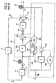
- In Figure 8, the disturbance d is input to adder 801 as a first input and the output of the
plant 802 is input as a second input to adder 801. The output ofadder 801 is the residual signal e online 803, which is measured byresidual sensor 826. - The residual 803 is input through an inverted input to a
second adder 804 which also receives an input from the probe signal n. The output ofadder 804 is sent as an input to controlfilter C 805 whose output c is sent to anactuation device 825. - The residual 803 is also provided as an input to probe
generation circuit 806, which can have the structure shown in Figure 4, for example. The probe signal n is generated at the output ofprobe generation circuit 806. The probe signal n is also sent to aDFT circuit 807 whose output is provided to a conjugate circuit 808a and anotherconjugate circuit 808b. - The output of
DFT circuit 807 is provided as an input tofirst multiplier 809. The output of conjugate circuit 808a is also provided as a second input tofirst multiplier 809. The output of conjugate circuit 808a is also provided as a first input to asecond multiplier 810. - The residual signal e is provided as an input to
DFT circuit 807a, whose output is provided as a second input tosecond multiplier 810. Adivider 811 receives a divisor input from the output offirst multiplier 809 and a dividend input from the output ofsecond multiplier 810. The output ofdivider 811 is an estimate of the quantity (PC)/(1+PC). As shown byline 830 at the output ofdivider 811, the estimated frequency response is transferred into theprobe generation circuit 806, equivalent toline 404 of Figure 4. - In figure 8, standard signal processing techniques are also used, but not illustrated to preserve clarity. That is, standard windowing and overlapping occurs before the inputs to the DFT's and ensemble averaging of the multiplier outputs takes place before the multiplier outputs are sent to the dividers.
- The output of
DFT circuit 807 is provided toconjugate circuit 808b, whose output is then provided as a first input tothird multiplier circuit 812.Third multiplier circuit 812 receives a second input from the output ofDFT circuit 807b which receives an input from the output ofcontrol filter 805. The output ofthird multiplier circuit 812 is provided as a divisor input tosecond divider circuit 813, which receives a dividend input from the output ofsecond multiplier circuit 810. - The output of
second divider circuit 813 is an estimate of the frequency response of the plant P. This estimate is provided tocircuit 814 which generates the weights forcontrol filter 805 therefrom. Techniques for this conversion are well known to those of ordinary skill in the art. See Athans et al., Optimal Control - An Introduction to the Theory and Its Applications, McGraw-Hill, Book Company, 1966; Maciejowski, Multi Variable Feedback Design, Addison-Wesley Publishing Company, 1989; Åström et al., Adaptive Control, Addison-Wesley Publishing Company, 1989. - The above feedback SISO system has been described with respect to a frequency domain implementation. It can be appreciated that the feedback technique can also be implemented in the time domain, using LMS algorithms, to achieve the same results according to the general principles described above.
- A purely time domain embodiment of the
probe generation circuit 353 of Figure 3 will now be described, in association with Figure 6. - In this embodiment, the residual e is passed through a bulk
time delay circuit 601 which delays a portion of the residual for a predetermined short time delay. The purpose of this bulk delay is to delay the input by a sufficient amount so that the output signal is uncorrelated with the input signal. The size of the time delay is chosen so as to be longer than estimates of the impulse response of the plant. Since the delay of thedelay circuit 601 is short, the amplitude at the output is substantially the same. That is, the residual has not had enough time to change substantially during the short time delay, yet sufficient time has elapsed (relative to the impulse response of the plant), to decorrelate the output ofdelay 601 with its inputs at all but tonal disturbance frequencies. Therefore, in the absence of tonals in the disturbance, the resultant output signal is phase-uncorrelated with the residual e. - As further shown in Figure 6, the output of the
delay circuit 601 is an inverted input to adder 602. The residual e is also input to an adaptive filter 603 whose output is presented as another input to theadder 602. The adaptive filter 603 has its weights adapted by means of anLMS circuit 604, which receives inputs from both the residual e and from the output of theadder 602. By providing such additional circuitry, tonal contributions in the residual e can be removed. - The output of
adder 602 is then input to a Scale by βcircuit 607 which scales theadder 602 output by the value β. Thecircuit 607's output is then input toadaptive filter 609,delay circuit 610 and plant estimate copy (P copy)filter 608.Filter 608 periodically receives copied weights fromfilter 357 of Figure 3. The output offilter 608 is input toLMS circuit 611. - The output of
delay 610 is fed to an inverted input ofadder 612 while the residual signal, e, is applied to a non-inverting input to adder 612. The output ofadder 612 is applied as a second input toLMS circuit 611. The LMS circuit controls the transfer function characteristics of theadaptive filter 609 so as to generate the probe signal, n, atoutput line 613. - The function of
delay 610 is to delay the output of the scale by βcircuit 607 for a time approximately equal to the time it takes for this output to pass through the various adaptive filters, so as to account for the transit time through such filters, as is generally well known in the art. See Widrow et al cited above. Such a delay period is typically much shorter than that ofbulk delay 601. - Accordingly, the circuits 607-612 perform the shaping function of Eqn. 6 by multiplying the output of
adder 602 by scale factor β and filtering the resultant signal by an estimate of the inverse of the plant. - Two variations on the probe generation circuit embodiments of Figures 4 and 6 will now be given with reference to third and fourth embodiments of Figures 5 and 7. The embodiments in Figures 5 and 7 provide alternate approaches to perform the functionality of
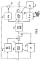
circuit elements circuit element 601 in Figure 6. - In embodiment three of Figure 5, the residual signal e is input to a finite impulse response (FIR) filter
coefficient determination circuit 502, which functions to select successive time records of the residual signal e for use as FIR filter coefficients byresidual filter circuit 503. The output of FIRfilter determination circuit 502 is provided as a control input toresidual filter circuit 503. The length of the time records selected bycircuit 502 should be chosen long enough to resolve the spectral features of the plant. This time record length, together with the sample rate of the controller, dictate the number of coefficients to be used inresidual filter 503. - The output of a
random number generator 504 is provided as a data input toresidual filter 503. The amplitude of the random noise from therandom number generator 504 is chosen so that the average power spectral density is 0 dB throughout the frequency range of concern. The output ofresidual filter 503, online 505, is the output of therandom number generator 504 filtered in the time domain byresidual filter 503. - Since the magnitude spectrum of the random noise is chosen to be flat, when such noise is passed through
residual filter 503, the magnitude spectrum of the output will approximate the magnitude spectrum of the residual. The output of theresidual filter 503 will be uncorrelated with the residual e by virtue of using therandom number generator 504 as input toresidual filter 503. - The output of
residual filter 503 online 505 can be used directly as an input to scale by βcircuit 607 in Figure 6. Alternatively, the output ofresidual filter 505 can be passed throughDFT circuit 501; then, as in Figure 4, the frequency domain result online 506 is passed toinverse filter 403,IDFT circuit 405, windowing and overlappingcircuit 406, and scale by βcircuit 407. - Figure 7 shows a fourth embodiment which is related to that presented in Figure 5. In Figure 7, however, the roles of the residual signal and random number generator are, in effect, reversed as compared to Figure 5. In Figure 7, the residual signal e is provided as a data input to scrambling
filter 703, whose weights are updated periodically through a control input from FIR filtercoefficient determination circuit 702, whose function is to select successive time records of the output of randomnumber generator circuit 704. The length of the time records selected bycircuit 702 and the amplitude of therandom number generator 704 are the same as those described forcircuits filter 703 is the residual signal e filtered in the time domain by scramblingfilter 703. - The output of the
scrambling filter 703 will be uncorrelated in phase but have substantially the same magnitude (power) spectrum as the residual signal e. - The output of the scrambling filter on
line 705 can be used directly as an input to the scale by βcircuit 607 of Figure 6. Alternatively, the output of the scrambling filter can be passed throughDFT circuit 701, and as in Figure 4, the frequency domain result online 706 is passed directly toinverse filter 403,IDFT circuit 405, window and overlappingcircuit 406, and scale by βcircuit 407. - Other techniques for decorrelating the phase spectrum of the residual yet maintaining the amplitude spectrum thereof, when generating the probe, could be derived by those of ordinary skill in the art. Such techniques are considered within the scope of coverage of the appended claims.
- For the feedforward case of Figure 3, it is known (see Eriksson) to allow for the possibility of a feedback transfer function between the output of the
actuator 16 and the response of thereference sensor 13. This transfer function is not shown in Figures 2 or 3 to preserve clarity. The probe generation procedures disclosed herein can be easily extended to and apply equally well to those systems where such a feedback transfer function is significant. - An algorithm for generating an "optimal" probe signal for the purpose of on-line plant identification within the context of feedforward and feedback algorithms applied to systems with time-varying plants has been disclosed. This algorithm differs from the more traditional techniques in that it is implemented as a closed-loop feedback path, and the spectral shape and overall gain of the probe signal are derived from measurements of the residual error sensor. The resulting probe signal maximizes the strength of the probe signal as a function of frequency, providing uniform SNR of the probe relative to the residual for estimating the plant transfer function. This SNR level is related to acceptable noise amplification through a simple expression.
- As a consequence of increasing the SNR for plant estimation relative to that achieved by using "white" noise probe signals for "non-white" residuals and plants, this new probe generation algorithm offers the possibility for more uniform broadband reduction and better system performance in the presence of slewing tonals in the disturbance.
Claims (38)
- A method of generating a probe signal for use in estimating the transfer function of a time-varying plant in an active noise or vibration control system, comprising steps of:(a) creating a residual signal by acoustically combining a response due to a disturbance with a response induced by the output of a controller of said control system;(b) determining a magnitude spectrum of said residual signal; and(c) generating a probe signal having a certain magnitude spectrum based on said determined magnitude spectrum of said residual signal.
- The method of claim 1, wherein said step (c) comprises sub-steps of:(c1) taking a Discrete Fourier Transform of the residual signal to form a complex spectrum consisting of a magnitude spectrum and a phase spectrum;(c2) randomizing the phase spectrum of the result of sub-step (c1), while preserving the magnitude spectrum thereof;(c3) shaping the complex spectrum of the result of sub-step (c2) by dividing said complex spectrum by an estimate of a transfer function from the probe signal to a residual sensor;(c4) taking the inverse Discrete Fourier Transform of the result of sub-step (c3); and(c5) scaling the result of sub-step (c4) by a gain factor.
- The method of claim 1, wherein said probe signal generated at said step (c) and the residual signal are input to a least mean square circuit whose output adapts coefficients of an adaptive filter to approximate a transfer function between the probe signal and the residual signal.
- The method of claim 3, wherein the adaptive filter is used within a filtered-x control algorithm to update coefficients of a control filter.
- The method of claim 4, wherein an output of said control filter is algebraically combined with said probe signal to create said output of said controller which is used in said step (a) to affect the residual signal.
- The method of claim 1, wherein the processing which takes place at said step (c) involves spectral shaping so that a substantially constant signal-to-noise ratio probe signal is generated throughout the controller bandwidth.
- The method of claim 1, wherein the processing which takes place at said step (c) includes making the resulting probe signal uncorrelated with the input residual signal.
- The method of claim 2, wherein an intermediate sub-step of windowing and overlapping the result of sub-step (c4) occurs between sub-steps (c4) and (c5).
- The method of claim 2, wherein sub-steps (c1) and (c4) involve instantaneous Discrete Fourier Transforms.
- The method of claim 1, wherein said step (c) involves inputting random noise through a filter.
- The method of claim 10, wherein, characteristics of said filter are adaptable based on the magnitude spectrum of said residual signal.
- The method of claim 1, wherein characteristics of said magnitude spectrum of said residual signal are determined using instantaneous Discrete Fourier Transform operations involving sequential time records.
- The method of claim 12, wherein the magnitude spectrum of said probe signal is determined for a particular time record from the magnitude spectrum of the residual signal during a previous time record.
- The method of claim 1, wherein an instantaneous Fourier transform operation occurs during the generation of said probe signal at step (c).
- The method of claim 14, wherein the results of said inverse Fourier transform operation are windowed and overlapped during generation of said probe signal at said step (c).
- The method of claim 15, wherein the results of windowing and overlapping are scaled by a factor related to a prescribed noise amplification limit throughout the controller bandwidth.
- A method of generating a probe signal for use in estimating the transfer function of a time-varying plant in an active noise or vibration control system, comprising steps of:(a) creating a residual signal by acoustically combining a response due to a disturbance signal with a response induced by an output of a controller of said control system;(b) determining a phase spectrum of said residual signal; and(c) generating a probe signal by randomizing the phase spectrum determined at said step (b).
- The method of claim 17, wherein an instantaneous Discrete Fourier transform operation occurs during the generation of said probe signal at step (c).
- The method of claim 18, wherein the results of said inverse Fourier transform operation are windowed and overlapped during generation of said probe signal at said step (c).
- The method of claim 19, wherein the results of windowing and overlapping are scaled by a factor related to a prescribed noise amplification limit throughout the controller bandwidth.
- An apparatus which generates a probe signal for use in estimating the transfer function of a time-varying plant in an active noise or vibration control system, the apparatus comprising:wherein said means for generating (353) comprises:(a) means (18) for creating a residual signal (e) by acoustically combining a response due to a disturbance with a response induced by an output of a controller (35) of said control system;(b) means (352) for feeding the residual signal (e) back into the controller (35); and(c) means (353) for generating said probe signal (n) inside of said controller (35) by processing the residual signal (e) fed back to the controller (35) at said step (b);(c1) means (401) for taking a Discrete Fourier Transform of the residual signal to form a complex spectrum consisting of a magnitude spectrum and a phase spectrum;(c2) means (402) for randomizing the phase spectrum of the result of element (c1), while preserving the magnitude spectrum thereof;(c3) means (403) for shaping the complex spectrum of the result of element (c2) by dividing said spectrum by an estimate of a transfer function from the probe signal (n) to a residual sensor;(c4) means (405) for taking the inverse Discrete Fourier Transform of the result of element (c3); and(c5) means (407) for scaling the result of element (c4) by a gain factor.
- The apparatus of claim 21 comprising:wherein said second addition circuit (359) receives an input from said residual signal (e);a control filter (351) receiving an input from said disturbance signal sensed by a reference sensor (13) of said active noise or vibration control system;a first algebraic addition circuit (355) receiving one input from an output of said control filter (351) and another input from said probe signal (n);a plant estimate filter (357) connected at a data input thereof to said probe signal (n), at a control input thereof to a first least mean square circuit (358) and at a data output thereof to a second algebraic addition circuit (359); anda third algebraic addition circuit (359a) receiving inputs from said residual signal (e) and an output of said plant estimate filter (357) and supplying an output to a second least mean square circuit (352);
wherein said first least mean square circuit (358) receives inputs from said probe signal (n) and an output of said second addition circuit (359);
wherein said second least mean square circuit (352) received an input from a copy (354) of said plant estimate filter (357) and provides an output to a control input of said control filter (351); and
wherein an output of said first algebraic addition circuit (355) is connected through an output line of said controller (35) to an actuator (16) of said active noise or vibration control system. - The apparatus of claim 21 or 22, wherein said means for generating (353) comprises:(c1) means (601) for delaying said residual signal;(c2) means (607) for scaling the result of element (c1) by a constant; and(c3) adaptive filter means (603) for adaptively filtering the result of element (c2) to output said probe signal (n).
- The apparatus of claim 23, in which said means for generating (353) further comprises:(c4) a delay (610) having an input connected to the output of said element (c2), and an output connected to an input of an algebraic adder (612) which receives another input from said residual signal (e);(c5) a filter circuit (609) having its input connected to an output of element (c2); and(c6) at least mean square circuit (611) having an input connected to an output of said element (c5), and another input connected to said algebraic adder (612) recited at said element (c4), and providing a control input to said adaptive filter means element (c3).
- The apparatus of claim 23, wherein said means for generating (353) further comprises:(c4) algebraic adder circuit (602) receiving an input from the output of means (c1) for delaying;(c5) adaptive filter (603) receiving an input from said residual signal and having an output connected to an input of said algebraic adder circuit (c4);(c6) least mean square circuit (604) receiving an input from said residual signal (e), and receiving another input from an output of said algebraic adder circuit (c4), and providing a control input to said adaptive filter (c5).
- The apparatus of claim 21, wherein said means for generating (353) comprises:(c1) a scrambling filter (703) receiving a data input from said residual signal (e) and a control input from a random number generator (704).
- The apparatus of any one of claims 21 to 26, in which the controller is of a feedforward type.
- The apparatus of any one of claims 21 to 26, in which the controller is of a feedback type.
- The apparatus of any one of claims 21 to 28, in which said means for generating operates in the time domain.
- The apparatus of any one of claims 21 to 28, in which said means for generating operates in the frequency domain.
- The method of claim 1, wherein the generated probe signal, the residual signal and the output of the controller are processed to provide an estimate of a transfer function between the probe and residual signals.
- The method of claim 3, wherein said plant transfer function estimation filter is used within a filtered-x algorithm to update the coefficients of a control filter.
- The method of claim 32, wherein an output of said control filter is algebraically combined with said probe signal to create said output of said controller which is used in step (a).
- The method of claim 2, wherein the processing of substep (c2) includes filtering the results of sub-step (c1) by an estimate of the inverse of a transfer function from the probe signal to the residual signal.
- The method of claim 3, wherein the processing of step (c) includes filtering a Fourier transformed residual signal by an estimate of the inverse of a transfer function from the probe signal to the residual signal, wherein said estimate is obtained by taking the Discrete Fourier Transform of weights of said adaptive filter, and inverting the transformed weights frequency by frequency.
- A method of generating cancelling vibratory energy with an output transducer for reducing oscillatory vibration in a selected spatial region in the presence of incident vibratory energy comprising:(a) sensing residual vibration in said region using a residual sensor and generating a corresponding residual signal;(b) filtering a signal derived from said residual signal using a first set of adjustable parameters which represent the inverse of a transfer function between said output transducer and said residual sensor;(c) further filtering the result of step (b) using a second set of adjustable parameters;(d) for determining an estimate of said transfer function, generating a probe signal as claimed in claim 1 or claim 17;(e) coherently detecting the contribution of said probe signal in said residual signal thereby to measure said transfer function;(f) adjusting said first set of parameters in accordance with the transfer function thereby measured;(g) independently adjusting said second set of parameters as a function of said residual signal and said probe signal thereby to continuously update said estimate of said transfer function;(h) sensing said incident energy upstream of said region thereby to generate a reference signal;(i) filtering said reference signal by said transfer function estimate from step (d);(j) further filtering said reference signal using a third set of adjustable parameters; and(k) adding the result of step (j) to said probe signal to create an actuation signal to said output transducer thereby progressively reducing the residual vibration in said region.
- A method as set forth in claim 37 wherein said second set of parameters is adjusted in accordance with a least mean square algorithm.
- A method as set forth in claim 37 wherein said third set of parameters is adjusted in accordance with a least mean square algorithm.
Applications Claiming Priority (2)
| Application Number | Priority Date | Filing Date | Title |
|---|---|---|---|
| US335936 | 1994-11-08 | ||
| US08/335,936 US5796849A (en) | 1994-11-08 | 1994-11-08 | Active noise and vibration control system accounting for time varying plant, using residual signal to create probe signal |
Publications (3)
| Publication Number | Publication Date |
|---|---|
| EP0712115A2 EP0712115A2 (en) | 1996-05-15 |
| EP0712115A3 EP0712115A3 (en) | 1997-10-22 |
| EP0712115B1 true EP0712115B1 (en) | 2002-09-04 |
Family
ID=23313860
Family Applications (1)
| Application Number | Title | Priority Date | Filing Date |
|---|---|---|---|
| EP95307979A Expired - Lifetime EP0712115B1 (en) | 1994-11-08 | 1995-11-08 | Active noise and vibration control system accounting for time varying plant, using residual signal to create probe signal |
Country Status (6)
| Country | Link |
|---|---|
| US (1) | US5796849A (en) |
| EP (1) | EP0712115B1 (en) |
| JP (1) | JPH08227322A (en) |
| AU (1) | AU697691B2 (en) |
| CA (1) | CA2162245A1 (en) |
| DE (1) | DE69528028T2 (en) |
Cited By (1)
| Publication number | Priority date | Publication date | Assignee | Title |
|---|---|---|---|---|
| WO2006076925A1 (en) * | 2005-01-24 | 2006-07-27 | Pinocchio Data Systems Aps | Sensor with coil and magnet and signal correction |
Families Citing this family (42)
| Publication number | Priority date | Publication date | Assignee | Title |
|---|---|---|---|---|
| GB9616755D0 (en) * | 1996-08-09 | 1996-09-25 | Kemp Michael J | Audio effects synthesizer with or without analyser |
| US6219427B1 (en) * | 1997-11-18 | 2001-04-17 | Gn Resound As | Feedback cancellation improvements |
| US7031949B2 (en) * | 1998-01-22 | 2006-04-18 | Mts Systems Corporation | Method and apparatus for generating input signals in a physical system |
| US6059274A (en) * | 1998-05-04 | 2000-05-09 | Gte Internetworking Incorporated | Vibration reduction system using impedance regulated active mounts and method for reducing vibration |
| ES2143952B1 (en) * | 1998-05-20 | 2000-12-01 | Univ Madrid Politecnica | ACTIVE ATTENUATOR OF ACOUSTIC NOISE THROUGH GENETIC ADAPTIVE ALGORITHM. |
| US6594365B1 (en) | 1998-11-18 | 2003-07-15 | Tenneco Automotive Operating Company Inc. | Acoustic system identification using acoustic masking |
| FR2786307B1 (en) * | 1998-11-19 | 2001-06-08 | Ecia Equip Composants Ind Auto | PILOTAGE SYSTEM FOR ELECTROACOUSTIC TRANSDUCER ACTIVE ANTI-NOISE FOR MOTOR VEHICLE EXHAUST SYSTEM |
| US6496320B1 (en) * | 2000-02-09 | 2002-12-17 | Seagate Technology Llc | Adaptive attenuation of multi-axis vibrational disturbance |
| US6487524B1 (en) * | 2000-06-08 | 2002-11-26 | Bbnt Solutions Llc | Methods and apparatus for designing a system using the tensor convolution block toeplitz-preconditioned conjugate gradient (TCBT-PCG) method |
| JP4901058B2 (en) | 2000-09-21 | 2012-03-21 | エムティエス・システムズ・コーポレーション | Multi-region convolver with taper function |
| EP1506353B1 (en) * | 2002-05-21 | 2006-11-08 | Bell Helicopter Textron Inc. | Variable stiffness support |
| US8746649B2 (en) | 2002-05-21 | 2014-06-10 | Textron Innovations Inc. | Variable stiffness support |
| JP4209247B2 (en) * | 2003-05-02 | 2009-01-14 | アルパイン株式会社 | Speech recognition apparatus and method |
| US6973403B1 (en) * | 2003-05-16 | 2005-12-06 | Bent Solutions Llc | Method and system for identification of system response parameters for finite impulse response systems |
| WO2006048815A1 (en) * | 2004-11-04 | 2006-05-11 | Koninklijke Philips Electronics N.V. | Encoding and decoding a set of signals |
| US7576606B2 (en) | 2007-07-25 | 2009-08-18 | D2Audio Corporation | Digital PWM amplifier having a low delay corrector |
| US7498781B2 (en) * | 2006-04-07 | 2009-03-03 | L&L Engineering Llc | Methods and systems for disturbance rejection in DC-to-DC converters |
| US20080221710A1 (en) * | 2006-10-13 | 2008-09-11 | General Electric Company | System and methods for reducing an effect of a disturbance |
| US7421354B2 (en) * | 2006-10-13 | 2008-09-02 | General Electric Company | Systems and methods for reducing an effect of a disturbance |
| EP1947642B1 (en) * | 2007-01-16 | 2018-06-13 | Apple Inc. | Active noise control system |
| US7728658B2 (en) | 2007-07-25 | 2010-06-01 | D2Audio Corporation | Low-noise, low-distortion digital PWM amplifier |
| US9142207B2 (en) | 2010-12-03 | 2015-09-22 | Cirrus Logic, Inc. | Oversight control of an adaptive noise canceler in a personal audio device |
| US8958571B2 (en) | 2011-06-03 | 2015-02-17 | Cirrus Logic, Inc. | MIC covering detection in personal audio devices |
| US9824677B2 (en) | 2011-06-03 | 2017-11-21 | Cirrus Logic, Inc. | Bandlimiting anti-noise in personal audio devices having adaptive noise cancellation (ANC) |
| US9318094B2 (en) | 2011-06-03 | 2016-04-19 | Cirrus Logic, Inc. | Adaptive noise canceling architecture for a personal audio device |
| US9318090B2 (en) | 2012-05-10 | 2016-04-19 | Cirrus Logic, Inc. | Downlink tone detection and adaptation of a secondary path response model in an adaptive noise canceling system |
| US9319781B2 (en) * | 2012-05-10 | 2016-04-19 | Cirrus Logic, Inc. | Frequency and direction-dependent ambient sound handling in personal audio devices having adaptive noise cancellation (ANC) |
| US9123321B2 (en) | 2012-05-10 | 2015-09-01 | Cirrus Logic, Inc. | Sequenced adaptation of anti-noise generator response and secondary path response in an adaptive noise canceling system |
| US9532139B1 (en) | 2012-09-14 | 2016-12-27 | Cirrus Logic, Inc. | Dual-microphone frequency amplitude response self-calibration |
| US9414150B2 (en) | 2013-03-14 | 2016-08-09 | Cirrus Logic, Inc. | Low-latency multi-driver adaptive noise canceling (ANC) system for a personal audio device |
| US9666176B2 (en) | 2013-09-13 | 2017-05-30 | Cirrus Logic, Inc. | Systems and methods for adaptive noise cancellation by adaptively shaping internal white noise to train a secondary path |
| US9704472B2 (en) | 2013-12-10 | 2017-07-11 | Cirrus Logic, Inc. | Systems and methods for sharing secondary path information between audio channels in an adaptive noise cancellation system |
| US10382864B2 (en) | 2013-12-10 | 2019-08-13 | Cirrus Logic, Inc. | Systems and methods for providing adaptive playback equalization in an audio device |
| US9846425B2 (en) | 2015-03-31 | 2017-12-19 | Bose Corporation | Retrieving pre-determined controller parameters to isolate vibrations in an authorized payload |
| US10026388B2 (en) | 2015-08-20 | 2018-07-17 | Cirrus Logic, Inc. | Feedback adaptive noise cancellation (ANC) controller and method having a feedback response partially provided by a fixed-response filter |
| US10013966B2 (en) | 2016-03-15 | 2018-07-03 | Cirrus Logic, Inc. | Systems and methods for adaptive active noise cancellation for multiple-driver personal audio device |
| DK3288285T3 (en) * | 2016-08-26 | 2019-11-18 | Starkey Labs Inc | METHOD AND DEVICE FOR ROBUST ACOUSTIC FEEDBACK REPRESSION |
| CN109657650A (en) * | 2019-01-15 | 2019-04-19 | 广东工业大学 | A kind of filtering method of random noise, device, medium and equipment |
| RU2748326C1 (en) * | 2020-02-11 | 2021-05-24 | Федеральное государственное бюджетное образовательное учреждение высшего образования Иркутский государственный университет путей сообщения (ФГБОУ ВО ИрГУПС) | System and method for controlling the vibration amplitude of a vibrating technological machine |
| CN111610752B (en) * | 2020-05-24 | 2021-07-27 | 西安交通大学 | Interpolation instruction evaluation method based on servo feeding system attenuation magnification |
| CN112444366B (en) * | 2020-12-08 | 2022-07-12 | 中国工程物理研究院总体工程研究所 | Random vibration test frequency-division mixed control method |
| CN114035626B (en) * | 2021-11-12 | 2022-10-04 | 中国科学院长春光学精密机械与物理研究所 | Vibration control device and control method thereof |
Family Cites Families (9)
| Publication number | Priority date | Publication date | Assignee | Title |
|---|---|---|---|---|
| US4122303A (en) * | 1976-12-10 | 1978-10-24 | Sound Attenuators Limited | Improvements in and relating to active sound attenuation |
| US4417098A (en) * | 1979-08-16 | 1983-11-22 | Sound Attenuators Limited | Method of reducing the adaption time in the cancellation of repetitive vibration |
| US4480333A (en) * | 1981-04-15 | 1984-10-30 | National Research Development Corporation | Method and apparatus for active sound control |
| US4677676A (en) * | 1986-02-11 | 1987-06-30 | Nelson Industries, Inc. | Active attenuation system with on-line modeling of speaker, error path and feedback pack |
| US4947435A (en) * | 1988-03-25 | 1990-08-07 | Active Noise & Vibration Tech | Method of transfer function generation and active noise cancellation in a vibrating system |
| US5402496A (en) * | 1992-07-13 | 1995-03-28 | Minnesota Mining And Manufacturing Company | Auditory prosthesis, noise suppression apparatus and feedback suppression apparatus having focused adaptive filtering |
| US5386477A (en) * | 1993-02-11 | 1995-01-31 | Digisonix, Inc. | Active acoustic control system matching model reference |
| JP3340496B2 (en) * | 1993-03-09 | 2002-11-05 | 富士通株式会社 | Estimation method of transfer characteristics of active noise control system |
| US5327496A (en) * | 1993-06-30 | 1994-07-05 | Iowa State University Research Foundation, Inc. | Communication device, apparatus, and method utilizing pseudonoise signal for acoustical echo cancellation |
-
1994
- 1994-11-08 US US08/335,936 patent/US5796849A/en not_active Expired - Lifetime
-
1995
- 1995-11-06 CA CA002162245A patent/CA2162245A1/en not_active Abandoned
- 1995-11-08 EP EP95307979A patent/EP0712115B1/en not_active Expired - Lifetime
- 1995-11-08 JP JP7324990A patent/JPH08227322A/en active Pending
- 1995-11-08 AU AU37702/95A patent/AU697691B2/en not_active Ceased
- 1995-11-08 DE DE69528028T patent/DE69528028T2/en not_active Expired - Fee Related
Cited By (1)
| Publication number | Priority date | Publication date | Assignee | Title |
|---|---|---|---|---|
| WO2006076925A1 (en) * | 2005-01-24 | 2006-07-27 | Pinocchio Data Systems Aps | Sensor with coil and magnet and signal correction |
Also Published As
| Publication number | Publication date |
|---|---|
| DE69528028D1 (en) | 2002-10-10 |
| AU3770295A (en) | 1996-05-16 |
| EP0712115A3 (en) | 1997-10-22 |
| JPH08227322A (en) | 1996-09-03 |
| AU697691B2 (en) | 1998-10-15 |
| US5796849A (en) | 1998-08-18 |
| EP0712115A2 (en) | 1996-05-15 |
| CA2162245A1 (en) | 1996-05-09 |
| DE69528028T2 (en) | 2003-04-30 |
Similar Documents
| Publication | Publication Date | Title |
|---|---|---|
| EP0712115B1 (en) | Active noise and vibration control system accounting for time varying plant, using residual signal to create probe signal | |
| US6683960B1 (en) | Active noise control apparatus | |
| EP0721179B1 (en) | Adaptive tonal control system with constrained output and adaptation | |
| Feintuch et al. | A frequency domain model for'filtered'LMS algorithms-stability analysis, design, and elimination of the training mode | |
| US4677676A (en) | Active attenuation system with on-line modeling of speaker, error path and feedback pack | |
| US4473906A (en) | Active acoustic attenuator | |
| US4903247A (en) | Digital echo canceller | |
| EP0695452B1 (en) | Frequency domain adaptive control system | |
| US9153226B2 (en) | Adaptive noise control | |
| KR970001736B1 (en) | Noise cancellor and its cancelling method | |
| US4122303A (en) | Improvements in and relating to active sound attenuation | |
| Elliott et al. | Adaptive control of flexural waves propagating in a beam | |
| EP1495463B1 (en) | Active noise control system in unrestricted space | |
| EP0654901B1 (en) | System for the rapid convergence of an adaptive filter in the generation of a time variant signal for cancellation of a primary signal | |
| NL9001016A (en) | DIGITAL ECHO COMPENSATOR WITH A DOUBLE-VOICE DETECTOR. | |
| JPS59133595A (en) | Active sound attenuator | |
| Zhang et al. | On comparison of online secondary path modeling methods with auxiliary noise | |
| US5440641A (en) | Active noise cancellation system | |
| US5627746A (en) | Low cost controller | |
| Kim et al. | Delayed-X LMS algorithm: An efficient ANC algorithm utilizing robustness of cancellation path model | |
| Meurers et al. | Model-free frequency domain iterative active sound and vibration control | |
| MT et al. | Acoustic feedback neutralization in active noise control systems | |
| Chen et al. | Evaluation of the convergence characteristics of the filtered-x LMS algorithm in the frequency domain | |
| WO1994029848A1 (en) | Error path transfer function modelling in active noise cancellation | |
| US5926405A (en) | Multidimensional adaptive system |
Legal Events
| Date | Code | Title | Description |
|---|---|---|---|
| PUAI | Public reference made under article 153(3) epc to a published international application that has entered the european phase |
Free format text: ORIGINAL CODE: 0009012 |
|
| AK | Designated contracting states |
Kind code of ref document: A2 Designated state(s): DE FR GB IT |
|
| PUAL | Search report despatched |
Free format text: ORIGINAL CODE: 0009013 |
|
| AK | Designated contracting states |
Kind code of ref document: A3 Designated state(s): DE FR GB IT |
|
| 17P | Request for examination filed |
Effective date: 19980417 |
|
| RAP1 | Party data changed (applicant data changed or rights of an application transferred) |
Owner name: BBN CORPORATION |
|
| 17Q | First examination report despatched |
Effective date: 20000215 |
|
| GRAG | Despatch of communication of intention to grant |
Free format text: ORIGINAL CODE: EPIDOS AGRA |
|
| RTI1 | Title (correction) |
Free format text: ACTIVE NOISE AND VIBRATION CONTROL SYSTEM ACCOUNTING FOR TIME VARYING PLANT, USING RESIDUAL SIGNAL TO CREATE PROBE SIGNAL |
|
| GRAG | Despatch of communication of intention to grant |
Free format text: ORIGINAL CODE: EPIDOS AGRA |
|
| GRAH | Despatch of communication of intention to grant a patent |
Free format text: ORIGINAL CODE: EPIDOS IGRA |
|
| GRAH | Despatch of communication of intention to grant a patent |
Free format text: ORIGINAL CODE: EPIDOS IGRA |
|
| GRAA | (expected) grant |
Free format text: ORIGINAL CODE: 0009210 |
|
| AK | Designated contracting states |
Kind code of ref document: B1 Designated state(s): DE FR GB IT |
|
| REG | Reference to a national code |
Ref country code: GB Ref legal event code: FG4D |
|
| REF | Corresponds to: |
Ref document number: 69528028 Country of ref document: DE Date of ref document: 20021010 |
|
| ET | Fr: translation filed | ||
| PLBE | No opposition filed within time limit |
Free format text: ORIGINAL CODE: 0009261 |
|
| STAA | Information on the status of an ep patent application or granted ep patent |
Free format text: STATUS: NO OPPOSITION FILED WITHIN TIME LIMIT |
|
| 26N | No opposition filed |
Effective date: 20030605 |
|
| PGFP | Annual fee paid to national office [announced via postgrant information from national office to epo] |
Ref country code: FR Payment date: 20031030 Year of fee payment: 9 |
|
| PGFP | Annual fee paid to national office [announced via postgrant information from national office to epo] |
Ref country code: GB Payment date: 20031031 Year of fee payment: 9 |
|
| PGFP | Annual fee paid to national office [announced via postgrant information from national office to epo] |
Ref country code: DE Payment date: 20031217 Year of fee payment: 9 |
|
| PG25 | Lapsed in a contracting state [announced via postgrant information from national office to epo] |
Ref country code: GB Free format text: LAPSE BECAUSE OF NON-PAYMENT OF DUE FEES Effective date: 20041108 |
|
| PG25 | Lapsed in a contracting state [announced via postgrant information from national office to epo] |
Ref country code: DE Free format text: LAPSE BECAUSE OF NON-PAYMENT OF DUE FEES Effective date: 20050601 |
|
| GBPC | Gb: european patent ceased through non-payment of renewal fee |
Effective date: 20041108 |
|
| PG25 | Lapsed in a contracting state [announced via postgrant information from national office to epo] |
Ref country code: FR Free format text: LAPSE BECAUSE OF NON-PAYMENT OF DUE FEES Effective date: 20050729 |
|
| REG | Reference to a national code |
Ref country code: FR Ref legal event code: ST |
|
| PG25 | Lapsed in a contracting state [announced via postgrant information from national office to epo] |
Ref country code: IT Free format text: LAPSE BECAUSE OF NON-PAYMENT OF DUE FEES;WARNING: LAPSES OF ITALIAN PATENTS WITH EFFECTIVE DATE BEFORE 2007 MAY HAVE OCCURRED AT ANY TIME BEFORE 2007. THE CORRECT EFFECTIVE DATE MAY BE DIFFERENT FROM THE ONE RECORDED. Effective date: 20051108 |