EP0626882B1

EP0626882B1 - Temperature scanning reactor

Info

Publication number: EP0626882B1
Application number: EP93902003A
Authority: EP
Inventors: Bohdan W. Wojciechowski; Norman M. Rice
Original assignee: Queens University at Kingston
Current assignee: Queens University at Kingston
Priority date: 1992-02-10
Filing date: 1993-01-27
Publication date: 1998-05-27
Anticipated expiration: 2013-01-27
Also published as: JPH07503405A; DE69318825T2; DE69318825D1; US5340745A; ATE166593T1; CA2128723A1; WO1993015829A1; EP0626882A1; ES2115753T3

Abstract

A method for rapidly collecting kinetic rate data from a temperature scanning reactor for chemical reactions. The method, which is particularly useful for studying catalytic reactions, involves ramping (scanning) of the input temperature to a reactor and recording of output conversion and bed temperature without waiting for isothermal steady state to be established.

Description

Field of Invention

This invention relates to a method and apparatus for determining rates of reaction in a chemical reactor system.

Background of Invention

The acquisition of kinetic rate data from a chemical reaction system is usually a laborious, time consuming and expensive undertaking. As a consequence, evaluation of catalysts and reaction conditions, in the chemical industry, for example, is often carried out with scanty data which does not allow for a full understanding of the system under study. Conventional methods generally include collecting iso-thermal conversion data at steady state for a number of feed rates. Because of operating requirements, such as waiting for steady state, start-up, shutdown etc., it is usually only possible to make 1-5 runs per day in any given system. At least 30 runs are needed over a range of 3 or 4 temperatures. About 8-10 space velocities are required at each temperature, and hence it will be seen that such a study will take about two months to complete. This time period may be considerably increased if repeat runs are required to verify catalyst stability over this length of time or to obtain a statistical measure of variance or if feed composition of reactant concentration are to be varied. Frequently, therefore, there may be as much as one person-year required for a full research study. There is, therefore, a considerable need for an improved method of acquiring kinetic rate data for chemical reactors.
Catal. Rev. -Sci.Eng., 25(2), 141-227 (1983) discloses temperature-programmed desorption (TPD) and temperature-programmed reaction (TPR) techniques for obtaining kinetic data using a stream swept reactor.

Object of Invention

An object of the present invention is to provide a method for determining kinetic rate data for chemical reactors which is at least an order of magnitude faster than conventional methods.

Another object of the present invention is to provide an improved apparatus for carrying out kinetic rate determinations for chemical reactions.

Brief Statement of Invention

Thus, by one aspect of this invention there is provided a method for rapid collection of kinetic rate data from a temperature scanning reactor selected from the group consisting of a plug flow reactor, an adiabatic reactor, a batch reactor, and a continuous stirred tank reactor, in which a feed stock is reacted under non-steady state conditions to form a conversion product comprising,

ramping the input temperature of said feed stock rapidly over a selected range of temperature,

continuously monitoring output conversion and output temperature and determining a rate of reaction under non-steady state conditions from said input and output temperatures, and output conversion.

By another aspect of this invention there is provided an apparatus for rapid collection of kinetic rate data for a chemical reaction, comprising,

a temperature scanning reactor selected from the group consisting of a plug flow reactor, a batch reactor and a continuous stirred tank reactor,

means to ramp a feed stock input temperature

means to continuously monitor output conversion and output temperature from said reactor; and

means to determine rates of reaction under non-steady state conditions from said input and output temperature, and output conversion. In a preferred embodiment the reactor is a plug flow reactor or a backmix reactor or a batch reactor.

Brief Description of Drawings

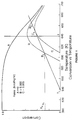
Figure 1 is a graph showing constant rate curves of methanol formation;

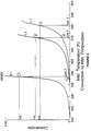
Figure 2 is a graph showing methanol conversion versus rate ^-1;

Figure 3 is a graph showing methanal conversion versus input temperature T_i at three constant space velocities or space times; WHSV = 0.1 (τ = 10); WHSV = 1.1 (τ = 0.91) and WHSV = 2.1 (τ = 0.48);

Figure 4 is a graph showing methanol conversion versus output temperature T_o at the same space velocities as in Figure 3;

Figure 5 are conversion curves X_A versus output temperature T_o at constant space velocity τ but varying input temperatures T_i superimposed on the equilibrium curve for the system;

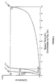
Figure 6 is a graph showing methanol conversion versus τ at constant input temperatures T_i T₁ = 536.7°K, T₂ = 570.7°K and T₃ = 581.3°K;

Figure 7 is a graph of simulated behavior of output temperature T_o as a function of input temperature in an adiabatic reactor for methanol synthesis operating under the conditions of Figure 1 at space velocities of Figure 3; and

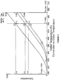
Figure 8 is a graph of methanol conversion versus temperature for the initial temperatures T₁ = 536.7°K, T₂ = 570.7°K and T₃ = 581.3°K, determined in Figure 3.

Figure 9 is a schematic diagram illustrating one embodiment of the automated temperature scanning reactor apparatus of the present invention

Detailed Description of Preferred Embodiments

Figure 1 shows an equilibrium curve for methanol synthesis at 333 atmospheres, two constant rate curves, and an adiabatic operating line, on coordinates showing the fraction converted versus the reaction-system temperature. Curve (A) corresponds to a rate of 10^-8 kmol(kg cat)^-1h^-1 and in essence represents the equilibrium for this system. Curve B corresponds to a rate of 2 x 10^-3kmol(kg cat)^-1h^-1, and , curve C corresponds to a rate of to 5 x 10^-3kmol(kg cat)^-1h^-1. The feed composition has CO:H₂:N₂:He:CO₂ in the ratio 1:5:1:2:1 at 333 atmospheres. The curves here and in the other figures were obtained using RESIM, an adiabatic reactor simulation program for the PC which uses the kinetics and parameters quoted by Capelli et al in "Mathematical Model for Simulating Behavior of Fauser-Montecatini Industrial Reactors for Methanol Synthesis", I. & EC. Proc. Des. Dev. II(2), (1972) p. 184-190. These data were obtained using established kinetics. An adiabatic reactor whose feed enters at the temperature where the operating line crosses X_A = 0 will yield an output at steady state which will invariably fall on this operating line. Exactly how far up this line the output will fall depends on the space velocity used. In the ideal case, all features of Figure 1 are fixed for each Pressure, catalyst, and feed composition including changes in inerts.

The equation of the operating line in this simplest case is XA = Cp T / - Hr Thus, X_A is directly proportional to T. This is true in systems which do not have significant secondary reactions or parallel reactions of different orders and do not lose heat to the reactor components or the surroundings. The matter becomes somewhat more complicated in the real world when the reactor and catalyst have finite heat capacities and heat loss may be unavoidable. In that case, the basic heat balance equation becomes: heat input = heat output + heat generated by reaction + heat accumulated in the reactor + heat lost to surroundings. Because a scanning reactor will be examined, which operates in a transient mode, the accumulation term cannot be ignored. By convention, the input condition is the enthalpy datum: i.e. heat input = 0.
The heat output term will depend on the composition of the products and can be written: heat output = Cp(To-Ti)(1-XA)+Cpp1(To-Ti)(XA-Xp)+Cpp2(To-TiXp) where only one primary product p1 and one secondary product p2 are postulated. More complex systems can be envisioned without changing the overall conclusions.

In accounting for heats of reaction, the heat of conversion of reactant to primary product p1 and the heat of conversion of that product to the secondary product p2 must be considered: heat generation by reaction = HriXA + HpiXp where X_p is the traction of conversion of the reactant A to secondary products p2 while X_A is the total fraction of reactant A converted. The subscripts ri and pi refer to heats of reaction of the feed A to p1 and p2 at the inlet temperature T_i.

In considering the accumulation terms, the heat capacity and mass of each of the components of the reactor must be considered. These will include reactor walls, the catalyst charge and any other items present in the reactor: accumulation = s Cpsmm Ts where the term T_s is the temperature difference between the reactor walls etc. and the reactants and the subscript s indicates the component of the reactor. The heat capacity C_ps is expressed in units commensurate with those of m, the quantity of a solid component in the reactor. Since at the beginning of a temperature scan the reactor is all at T_i, T_s is a function of both time and position in the reactor.

Finally, heat losses from the reactor will take the form: heat loss = f hfSf Tf where h is the heat transfer coefficient, S is the heat transfer surface and T_f is the driving force due to temperature difference between the reactor component f and its surroundings. Again, T_f will be a function of time. These terms are collected to present a more complete form of equation 1 XA = Cp T +s Hp2Xp + f msCps Ts + ΣhfSf Tf - Hr2 It can be seen that Equation 1a reduces to Equation 1 when all of the following are true:

a) secondary reaction does not occur and X_p = 0

b) the heat capacity of the reactor is very small and C_ps → 0 or when heat transfer to the reactor material is very slow, or at steady state when T_s = 0

c) heat loss from the reactor components is small because

1) h_f are all very small

2) T_f is minimized by appropriate instrument design.

Under appropriate conditions, there will exist a unique operating line for every real reactor under a prescribed set of operating conditions and, in the case of the adiabatic reactor, it is obvious that the operating line is unique. The reaction rate curves, on the other hand, are independent of the heat effects and will depend only on temperature, feed composition, catalyst activity and pressure regardless of adiabaticity.

To get from the input condition shown as T₁ in Figure 1 to an output condition at B₁ using a plug flow reactor (PFR) will require a certain space time τ_B1. To reach condition C₁ from T₁ will require a different space time τC₁ with τC₁ > τB₁, etc. In a PFR, each point on the operating line is reached at a unique space time.

At the space velocity which results in τB₁, an output conversion X_AB1 will be achieved which will be changing at a rate corresponding to constant rate curve B, regardless of how this point is reached either along an ideal operating line given by equation 1 or along a more complicated path given by equation 1a or its elaborations. If space velocity is decreased, i.e. increase τ to τC₁, condition C₁ will be reached which is the maximum rate achievable on the operating line starting at T₁ and lies on constant rate curve C. Further increases in τ will result in higher conversions but at decreasing rates. On the way to equilibrium conversion on Curve A, curve B will be encountered again at condition B₂. The rate at B₁ and B₂ will be the same; at B₁ it will occur at low conversion and low temperature while at B₂ it will take place at high conversion and high temperature. Thus, measurement of the rates of reaction and conversions along such operating lines, enables construction of curves such as those shown in Figure 2.

Figure 2 shows a plot of the reciprocal rate versus conversion. From reactor design, theory, this information is used to size the reactor using the general equation: τ = CA0 0 XAf dxA|-rA . The area under the curve on Figure 2 between X_A = 0 and XA = XAf is 0 XAf dXA/-τA = τ/CAO . Equation 3 is valid whether the temperature of the system is constant or not. At constant temperature T: dXA/-τA|T = dτ/CA0|T or rearranging CA0 dXA/dτ|T = -τA|T . In order to obtain the rate at a given reaction temperature, the value of dX_A/dτ at that temperature is required. This information is routinely obtained in isothermal reactors, however, in PFRs, it may be most readily obtained, not by the procedure of incrementing the input space velocity, but by the simple procedure of ramping the input temperature at constant space velocity and composition, so as to scan an input temperature range from T_min to T_max and observe the conversion X_A at each condition.

The temperature scanning procedure is equivalent to investigating the output condition, at constant τ, on a succession of operating lines, as identified for the 2.1 WHSV curve on Figures 3 and 8 by points 3, 4, and 5. In Figure 3 a series of curves showing how X_A varies with the input temperature (T_i) as a result of scans for various constant values of τ, all at constant composition and pressure are shown. In practice, the input temperature is ramped until a preset maximum output temperature T_omax is recorded, to protect the reactor or the catalyst or simply to avoid reaching equilibrium conversion. After each scan, a data set consisting of triplets of readings of T_i, T_o and X_A at corresponding times during the scan is produced.

Such a data set was used to produce Figure 3 and can also be plotted in another form by plotting X_A versus T_o as shown in Figure 4. There is little point in pushing the inlet temperature too high as can be seen by superimposing Figure 4 on the rate curves of Figure 1 as shown in Figure 5. At input temperatures above a certain value, the equilibrium condition at the output, as indicated by the uppermost curve corresponding to WHSV = 0.1 is obtained. To investigate the kinetics of a reaction it is preferable to stay below, in fact well away from equilibrium.

In Figure 3, it can be seen that at any T_i values of X_A at as many values of τ as have been investigated can be obtained. In fact, many sets of such values at various inlet temperatures T_i, within the range of temperature studied can be obtained. Each such set can then be plotted as shown in Figure 6. The curves on Figure 6 are curves of conversion vs space time along operating lines starting at the various temperatures indicated. Differentiating the curves on Figure 6 produces dX_A/dτ at constant T_i and the information necessary to plot Figure 2. These are the rates which might be observed along an operating line starting at a given T_i if such a measurement were possible. The functional form of the operating line does not matter, as long as there exists a unique operating line for the conditions used.

From a family of curves such as those shown on Figure 2, the constant rate curves shown on Figure 1 can be constructed and hence all the information necessary for kinetic model fitting can be obtained. Experimental operating lines which can be used to evaluate the heat effects involved in the reaction can also be generated. For each X_A and T_i from Figure 3, a T_o can be read off, for the same τ, on Figure 4. This give a set of values of X_A and T_o at constant T_i. This data, when plotted as X_A vs T_o, will produce an experimental operating line.

If the experimental operating lines are almost straight, it can be assumed that the reaction products either are stable or do not have a significant heat of reaction during conversion to secondary products and that the heat loss and accumulation terms in equation 1a are unimportant. If the primary products react endothermally, the operating lines will be concave or tend to curl up. Large temperature effects in the heat capacities of products and reactants can also induce curvature in the operating lines. Other effects, such as heat transfer from the reactants to the catalyst or other materials in the reactor, will also induce a concave curvature of the operating lines in ways which in some cases can be quantified. Careful determination of reactor and catalyst heat capacities, of the heats of reaction for secondary reactions and minimization of heat loss in order to approach adiabatic conditions, can be used to derive a fuller description of the observed operating lines. The time-dependent terms of Equation 1a can also be evaluated by suitable instrument calibration procedures.

Even if nothing of the chemistry, thermodynamics or kinetics of the reaction is known, useful qualitative information about the reaction from data such as that shown in Figure 3 can be obtained. A Temperature Scanning Reactor (TSR) run plotted on the coordinates of Figure 3, when repeated on a different catalyst formulation, will show if the new catalyst is more active. The curves for the more active catalyst would lie above those for the less active. There is nothing to prevent two such curves, obtained on different catalysts, from crossing. This would simply indicate that the activation energies or mechanisms of reaction are different on the two catalysts, thereby providing additional useful information.

Experimental Procedure

An automated temperature scanning reactor 1 apparatus, as seen in Figure 9, can be set up in such as way that feed space velocity is maintained at a constant value, while reactant input temperature T_i at gas inlet 2 is ramped over a range of temperatures ending at some input temperature which results in a maximum allowed output temperature T_omax at gas outlet 3. The reactor 1 is then cooled, equilibrated at its initial input temperature T_imin and a new space velocity selected. The ramping of the temperature is repeated and stopped again when T_omax is reached. The procedure is repeated at as many space velocities as necessary, say about 10. The data gathered during each temperature scan consist of a set of T_i and corresponding T_o. If necessary, X_A is followed at the same time using on-line FTIR or MS analysis using a mass spectrometer 4 or other analytical facility for continuous monitoring of output conversion. In the best of cases, X_A may be related to T by calculation or by auxiliary experiments.

An experimental setup which approaches an ideal adiabatic reactor is useful for simplifying the measurement of X_A. In the ideal case, equation 1 will apply and X_A can be calculated from the difference between T_o and T_i. Departures from the adiabatic condition may necessitate the evaluation of series of temperature scans will yield for each space velocity a set of data consisting of the triplets T_i, T_o and X_A.

The data logging, temperature scanning and space velocity changes can all be put under the control of a computer 5. The experimental data consisting of sets of T_i and T_o and X_A at various will be logged numerically or presented graphically on recorder 6 to look like the curves shown in Figure 3, 4 or 7. These are the raw data presentations.

Using X_A data in the form shown in Figure 4, one or more output temperatures, at which isothermal rate constants are required are selected. In this example T = 640K is selected and it is found that the output conversions which occur at this temperature at the three space velocities of 0.1, 1.1 and 2.1 hr ^-1 are 0.39, 0.27 and 0.23. The corresponding conditions are labeled with circled 1, 2 and 3 for cross reference with other figures. These conversions are used in Figure 3 to find the input temperatures T_i which lead to these output conditions.

Now, the values for T_i thus determined lie at X_A = 0 on the operating lines shown on Figure 8 and X_A values form the figure 4 should all occur at 640K on the appropriate operating lines, as they clearly do.

If enough scans at various values of τ are made it is possible to draw curves such as those shown in Figure 6 to an arbitrary degree of precision by plotting X_A vs τ at each T_i. Figure 6 is simply a new representation of the experimental data obtained by remapping the raw data. Differentiating the curves on Figure 6 produces values for plotting Figure 2. Figure 2 is also derived from the experimental data and represents the rates of reaction along operating lines. Because it is necessary to differentiate the data on Figure 6 to obtain Figure 2, it is clear that enough runs with appropriate values of τ to make the numerical differentiation accurate will be required.

All that remains is to read the rates from the appropriate curves on Figure 2 or from a plot of X_A vs rate for the X_A values at the 640K selected on Figure 4. This produces a set of rates and corresponding conversions at the selected reaction temperature T = 640K. This isothermal rate data can be treated in a conventional fashion by fitting it to postulated kinetic models using graphical or statistical methods.

If the feed contains more than one component, this procedure should be repeated at a number of feed compositions in order to determine the kinetic effect of each component in the system. This can be automated and need not complicate data gathering or interpretation beyond what is described above.

Data Handling Formalism

All of the above can be readily programmed on a computer by applying the following transformations of the basic T_i, T_o and X_A data set.
Let

T_i(i): be the set of input temperatures with i = 1 to m
τ (j): be the set of space times (or 1/WHSV) with j = 1 to n
T_o(i,j): be the set of output temperatures
X_A(i,j: be the set of output conversions.

In practice the set of input and output temperatures will be dense, and linear interpolations between adjacent measured results in the i direction can be applied. The space velocity set will, for reasons of economy of effort, be much sparser and necessitate second order interpolations.

When the rate of reaction is considered, and if the data in the j direction are sparse, a quadratic interpolation might be used:

for all j = 2, ..., n-1 while for the end members of the set -r(i,1) = CAO X(i,2) - X(i,1)τ2 - τ1 + X(i,3) - X(i,1)τ3 - τ1 - X(i,3) - X(i,2)τ3 - τ2 and -r(i,n)=CAO X(i,n) - X(i,n-1)τn - τn-1 + X(i,n) - X(i,n-1)τn - τn-2 X(i,n-1) - X(i,n-2)τ3 - τ2 . In the above, C_AO is the initial feed concentration of the base component A whose conversion we are tracking. The formulas can be simplified somewhat by carrying out the experimental program so that for all j the step size in space time is the same: τj - τj = constant Alternately spline functions may be fitted and differentiated directly.
A complete table of rates r(i,j) can therefore be assembled in one-to-one correspondence with the measurements of T_o and X_A. This can then be used in a program which simultaneously evaluates all rate constants and their Arrhenius parameters.

If the density in the i direction is high, rates at any desired temperature can be interpolated within the range of the scan by linear interpolation and rate constants at selected isothermal conditions can be evaluated. In the linear case, an output temperature T_o(k,j) such that k is constant for all j is selected. Output temperatures which bracket the desired T_o at each τ are identified. Let these output temperatures be: lower value = To(1,j) higher value = To(h,j) where 1 and h correspond to actually measured values of T_o at conditions 1 and h. Each of these conditions has a corresponding rate r(1,j) and r(h,j). These can be linearly interpolated to give the new rates at k enlarging the set of available temperature conditions to m + 1: -r(k,j) = r(1,j) + To(k,j) - To(1,j)To(h,j) - To(1,j) [r(h,j) - r(1,j)]. The corresponding conversion is: XA(k,j) = XA(1,j)+ To(k,j) - To(1,j)To(h,j) - To(1,j) [XA(h,j) - XA(1,j)] In this way, a set of r(k,j) and corresponding X_A(k,j) values is calculated. Such sets of isothermal rates and corresponding conversions can be obtained at many temperatures. They can be processed further by well-known means to determine the best kinetic expression and its parameters using model discrimination techniques or, in cases when the rate expression is known, to produce rate parameters, activation energies, etc. As Figure 6 makes plain, the important experimental requirement is that enough space velocities must be used to define the curves of X_A versus τ in sufficient detail so that equations 8 - 10, or other fitting procedures, are applicable within tolerable limits. The policy of keeping (τ_j - τ_j-1) constant, though it simplifies computation, may require a large number of experiments to determine each X_A versus τ curve with adequate precision. In general, it may be best to vary (τ_j - τ_j-1) in order to minimize experimental effort and define each curve in as much detail as is necessary.

If each value of τ can be scanned in 30 minutes, and if 10 values of τ will suffice for a given investigation, and if it takes 30 minutes to reset T_{i min} and change the space velocity, then a typical completely automated kinetic investigation using the TSAR should produce a best-fit model and its full set of kinetic parameters in something like a 24-hour period of automated data collection.

The data will yield, in principle, an unlimited number of isothermal data sets of r_A and X_A between the limits of the scans with something in the order of 10 space velocities at each temperature. This abundance of information, available in 24 hours, should be compared to the small set of data normally generated in months-long kinetic investigations.

It will be appreciated that while this invention has been described with reference to a plug flow reactor (PFR) and particularly an adiabatic plug flow reactor (APFR), the principles thereof are equally applicable to Continuous Stirred Tank Reactors (CSTR) and Batch Reactors.

The operating procedures for the CSTR are the same as for the Plug Flow Reactor i.e. ramping input temperature and recording output temperature and conversion. The equations required to calculate rates from CSTR data are simpler than those described above for the PFR and this alone may make the use of a suitable CSTR preferred in the application of the experimental methods described above. The CSTR has other attractive features such as better temperature control and lack of thermal gradients which may make its application even more attractive.

In the case of Batch Reactors it is possible to maintain uniform temperature in the reactor while ramping the temperature over a selected range. The advantage of this type of reactor is that high pressure reactions or the reactions of solids may be investigated by ramping the temperature of reactor contents while observing the degree of conversion and the temperature of the contents. This operation is advantageous in cases where kinetics are at present being studied in batch autoclaves or in atmospheric pressure batch reactors.

The rate of data acquisition can be doubled over and above that available by means of the procedures described above by the simple expedient of ramping the temperature up to a selected limit at a fixed space velocity and, instead of cooling back to the initial condition before the next data acquisition run, proceeding to change the space velocity at the high temperature limit and cooling the reactor with feed being supplied at the new space velocity. Data can then be acquired both on the temperature up-ramp and on the down-ramp. The space velocity is once again changed at the bottom of the ramp and a new up-ramp initiated. In this procedure there is essentially no "idle time" for the reactor and productivity of the apparatus is maximized.

Note also that the methods outlined in the above are applicable with minor alterations to cases where the reactor is not operated in an adiabatic manner, cases where the volume of the reacting mixture changes due to conversion and a number of other complications which are known to occur in such systems.

Claims

A method for rapid collection of kinetic rate data from a temperature scanning reactor selected from the group consisting of a plug flow reactor, an adiabatic reactor, a batch reactor, and a continuous stirred tank reactor, in which a feed stock is reacted under non-steady state conditions to form a conversion product comprising,

ramping the input temperature of said feed stock rapidly over a selected range of temperature,

continuously monitoring output conversion and output temperature and determining a rate of reaction under non-steady state conditions from said input and output temperatures, and output conversion.
An apparatus for rapid collection of kinetic rate data for a chemical reaction, comprising,

a temperature scanning reactor selected from the group consisting of a plug flow reactor, a batch reactor and a continuous stirred tank reactor,

means to ramp a feed stock input temperature

means to continuously monitor output conversion and output temperature from said reactor; and

means to determine rates of reaction under non-steady state conditions from said input and output temperature, and output conversion.